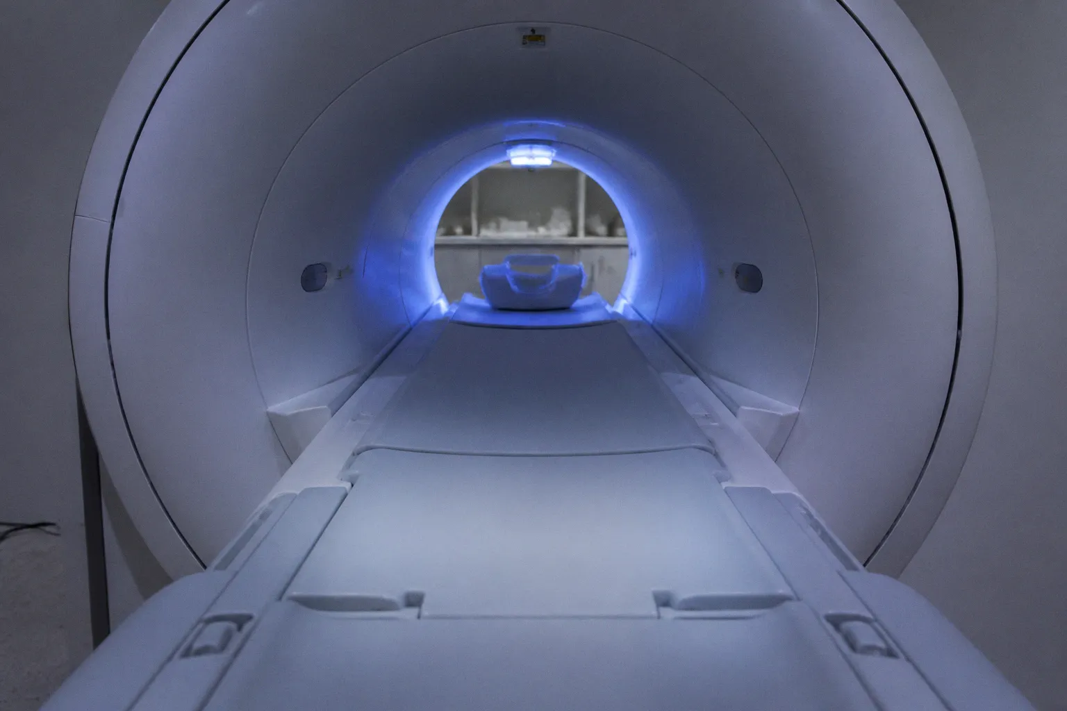
It is the gradient system itself: rapidly switched magnetic fields generate mechanical forces in the gradient coils and surrounding structures. The scanner is converting electrical timing into vibration, and vibration into pressure waves.
Silent MRI pulse sequences reduce that pressure by changing the timing mathematics of acquisition. They slow gradient transitions, lower slew rates, reshape readout trajectories, or remove the conventional delay before signal sampling through zero-TE methods. The result can be clinically valuable. It is not free. Acoustic noise reduction in MRI gradients consumes one or more of the quantities that normally make MRI efficient: sampling bandwidth, spatial resolution, contrast stability, signal-to-noise ratio, or scan time.
A quiet sequence is not a quieter version of the same acquisition. It is a different allocation of gradient time, sampling time, and signal quality.
The physics of acoustic noise in high-field MRI
MRI acoustic noise is a hardware consequence of pulse-sequence demand. The gradient coils must produce rapidly changing magnetic fields in three spatial directions. Those fields interact with current-carrying conductors and the static magnetic field. The mechanical response is proportional to the forces generated during switching. The gradient assembly moves. The scanner structure transmits that motion. The patient hears the result as the familiar knocking, buzzing, and high-frequency mechanical modulation of a scan.
The critical parameter is not merely the peak gradient amplitude. It is the rate at which the gradient changes. Slew rate describes that transition: how quickly the gradient moves from one amplitude to another. Aggressive slew rates support short echo spacing, rapid phase encoding, compressed readouts, and high temporal efficiency. They also produce sharper mechanical excitation.
This is why two sequences operating on the same scanner can have radically different acoustic profiles. The static field strength may be identical. The gradient hardware may be identical. The acoustic output changes because the sequence applies a different gradient trajectory.
Standard clinical MRI noise commonly occupies the 80–110 dB(A) range. Some high-field sequences reach approximately 130 dB at peak conditions. These figures are not a universal property of the magnet. They depend on:
- gradient amplitude and slew rate;
- repetition of switching events;
- frequency content of the waveform;
- echo-planar or fast spin-echo architecture;
- acceleration and parallel-imaging settings;
- gradient direction and physical coupling within the scanner;
- bore, room, and patient-positioning acoustics.
The scanner does not need to be “loud” in every sequence. It needs to execute certain gradients quickly. The noise is the audible signature of that execution.
Why high-field systems make the problem harder
Higher field strength does not automatically mean higher acoustic output. The relationship is indirect. High-field MRI tends to support more demanding protocols: higher spatial resolution, susceptibility-sensitive imaging, advanced diffusion, functional MRI, spectroscopy, and rapid three-dimensional readouts. These protocols often place heavier demands on the gradient subsystem.
At 3 Tesla, a demanding neurological sequence can therefore produce substantial acoustic pressure even though the scanner is operating within ordinary clinical specifications. The problem is not a failure of field stability. It is a conflict between fast gradient motion and mechanical response.
A sequence designer has several ways to reduce that response. None is equivalent to turning the gradients off. The system must still encode spatial information. The design task is to preserve the required k-space trajectory while avoiding the most mechanically disruptive transitions.
Gradient waveform engineering: from slew rates to zero TE
The most direct approach to acoustic noise reduction in MRI gradients is to reshape the gradient waveform. Instead of commanding abrupt transitions, the sequence applies gentler ramp-up and ramp-down profiles. The peak slew rate falls. The mechanical excitation is reduced.
That intervention changes the acquisition timing immediately. A longer ramp consumes part of the repetition or echo interval. The sequence may need to extend the readout, reduce the number of sampled points, alter the bandwidth, or accept a longer total examination.
The trade-off is sequence-specific. A turbo spin echo acquisition does not respond to waveform modification in the same way as a gradient echo acquisition. An echo-planar sequence has its own sensitivity because the readout repeatedly reverses the frequency-encoding gradient. A three-dimensional anatomical sequence may tolerate a different compromise, particularly if the available contrast and scan time are less constrained.
Conventional gradient moderation
Quiet versions of conventional sequences preserve the basic acquisition family but modify the gradient timing. The waveform becomes less abrupt. Slew rates are reduced. Gradient switching is distributed over a longer interval.
This approach has an important advantage: the sequence remains recognizable to the clinical protocol. Contrast behavior can remain close to the original implementation. The cost appears elsewhere:
- longer echo spacing;
- longer repetition or acquisition time;
- reduced temporal efficiency;
- altered susceptibility to motion;
- reduced spatial resolution if the matrix or bandwidth is constrained;
- lower SNR if the usable sampling window is shortened.
The resulting sequence is quieter, but not necessarily silent. The word “silent” is operational shorthand. It does not mean zero acoustic output under all conditions.
Zero-TE acquisition
Zero-TE techniques take a more structural approach. Conventional MRI sequences often contain a delay between radiofrequency excitation and the start of readout. That delay is incompatible with very rapidly decaying signals. Zero-TE methods begin sampling essentially immediately after excitation, using a three-dimensional radial or center-out trajectory.
GE Silenz and Siemens PETRA are the relevant examples in the supplied clinical and vendor data. Both use acquisition strategies that reduce the need for abrupt gradient behavior associated with conventional readouts. The acoustic profile can approach the background level of the scanner room.
The engineering is not trivial. Immediate sampling imposes strict demands on transmit-receive switching, gradient timing, eddy-current behavior, trajectory calibration, and reconstruction. A radial or center-out trajectory also changes the distribution of sampling in k-space. Motion behavior, undersampling artifacts, and contrast implementation must be evaluated as part of the sequence rather than treated as secondary details.
The benefit is substantial in appropriate protocols. In a clinical trial on a 3 Tesla system, a 3D T1-weighted Silenz sequence produced mean acoustic noise of 68.8 dB, compared with 104.65 dB for a standard BRAVO sequence. The measured Silenz level was effectively aligned with the reported scanner-room background of 68.73 dB.
That is a reduction of approximately 36 dB in the measured comparison. It is not a minor adjustment to the auditory environment. It is a change from dominant scanner noise to near-background operation.
But the acquisition still has to pay. The cost may appear as altered contrast, longer scan duration, reduced resolution, or a signal penalty. The quietness is real. So is the engineering compromise.
The relevant question is not whether a sequence is quiet. It is which image property was spent to make it quiet.
Quantifying the silent MRI scan time penalty
The phrase “scan time penalty” is often used too casually. It does not represent one universal percentage. The increase depends on the sequence family, target resolution, acceleration, desired contrast, reconstruction method, and SNR requirement.
The same gradient modification can be tolerable in a routine three-dimensional anatomical acquisition and unacceptable in a time-critical functional or diffusion protocol. In one case, an extra acquisition interval may be absorbed by protocol design. In another, it directly reduces temporal resolution or increases motion exposure.
Low-noise optimization generally introduces an approximate 10% SNR penalty in the available implementations described by the research material. That figure should not be treated as a constant for every scanner or sequence. The practical impact depends on how the protocol compensates. If the operator increases averages, enlarges voxel volume, reduces bandwidth, or extends the scan, part of the loss can be recovered. Each compensation consumes a different resource.
The signal equation does not provide a free correction. If the sequence loses effective sampling time, SNR degrades. If the voxel is made smaller, SNR degrades. If the bandwidth is increased to preserve timing, SNR generally degrades. If averages are added, scan time rises. The acquisition is a constrained system.
What is actually being traded
| Acquisition property | Effect of quieter gradient design | Practical consequence |
|---|---|---|
| Slew rate | Reduced during ramp-up and ramp-down | Lower mechanical excitation, but less aggressive encoding |
| Readout duration | Often extended | Longer repetition or echo timing; possible scan-time increase |
| Sampling window | Can be shortened or redistributed | Lower SNR or altered spatial-frequency coverage |
| Spatial resolution | May be reduced to preserve time | Small structures become less separable |
| Contrast timing | Can shift with TE, TR, or echo spacing | Tissue contrast may no longer match the standard sequence |
| Total scan time | Often increases, depending on implementation | Greater exposure to patient motion |
| Acoustic output | Falls, sometimes dramatically | Better tolerance for noise-sensitive examinations |
The 10% SNR penalty is modest only when the original protocol has sufficient signal margin. In low-SNR applications, a 10% loss can move a marginal sequence below the threshold required for reliable segmentation, lesion conspicuity, quantitative mapping, or longitudinal comparability.
This matters particularly in neuroimaging. A quiet T1-weighted scan may remain diagnostically useful while producing contrast behavior that differs from the established protocol. A research pipeline trained on conventional images may respond to the new intensity distribution, resolution profile, or artifact pattern in ways that are not obvious from visual inspection.
Noise reduction versus image quality
Image quality is not a single number. A sequence can preserve visual sharpness while changing contrast-to-noise ratio. It can preserve CNR while changing spatial resolution. It can preserve both on a selected phantom or volunteer dataset while increasing sensitivity to motion during the longer acquisition.
The more useful question is whether the quiet sequence preserves the metric required by the application.
For a clinical anatomical examination, that may be lesion conspicuity and robust contrast. For a segmentation pipeline, it may be intensity consistency and geometric fidelity. For diffusion, it may be directional sampling stability and distortion behavior. For functional MRI, it may be temporal SNR and the preservation of task-related fluctuations.
A quiet acquisition that improves patient tolerance but shifts the statistical properties of the images is not automatically a drop-in replacement. It requires protocol validation.
Clinical performance of Quiet Suite and PETRA sequences
Vendor implementations package the waveform and reconstruction changes into clinically deployable suites. Siemens Quiet Suite uses QuietX gradient modifications and the zero-TE PETRA sequence. The reported reduction in acoustic sound pressure reaches up to 97% during neurological and orthopedic examinations.
A reduction expressed as a percentage can obscure the physical scale of the change. Sound pressure is logarithmic. The audible and measured result depends on the baseline sequence, frequency weighting, microphone position, bore geometry, and the exact examination protocol. A 97% reduction in sound pressure should therefore be read as an implementation-specific performance claim, not a universal property of every quiet scan.
The clinical value is clearest in examinations where acoustic burden interferes with the acquisition itself. Lower sound can reduce the need for aggressive hearing protection, improve communication, and make certain protocols more tolerable. It can also be relevant when patient movement is associated with acoustic stress. But the sequence does not remove all motion. It does not eliminate the need for immobilization. It does not repair a poor acquisition strategy.
Silenz: near-ambient operation with a different readout model
The Silenz result at 3 Tesla is technically significant because it places the measured noise near the room background: 68.8 dB versus 68.73 dB ambient. The standard BRAVO comparison measured 104.65 dB.
The relevant point is not the product label. It is the acquisition architecture. Zero-TE sampling changes when the system begins collecting signal and how the trajectory traverses k-space. That affects the reconstruction problem. Image formation must account for the non-Cartesian trajectory, gradient delays, and system imperfections. The lower noise is achieved through a different signal-processing path, not by muting a conventional sequence after the fact.
This distinction matters for software teams. A pipeline that assumes Cartesian sampling, conventional intensity behavior, or a specific artifact distribution may require adaptation. A quiet sequence can be clinically acceptable and computationally inconvenient at the same time.
PETRA: silence constrained by sampling and reconstruction
PETRA uses a zero-TE strategy with radial sampling near the center of k-space and a mechanism for handling portions of k-space that cannot be acquired in the same way as the rest of the trajectory. That architecture supports very short effective echo times and low acoustic output, but it also increases dependence on trajectory fidelity and reconstruction choices.
Radial sampling can provide useful motion behavior because information is distributed across projections rather than concentrated in a single phase-encoding direction. It does not make motion irrelevant. Inconsistent motion during a long acquisition can still produce blurring, intensity variation, and reconstruction artifacts.
The sequence remains a mathematical engine. It does not know that the patient is anxious, that the protocol is behind schedule, or that a radiologist expects identical contrast to a conventional acquisition. The reconstruction receives signal along a trajectory. If that trajectory changes, the image statistics change with it.
Algorithmic optimization for TSE and GRE protocols
Zero-TE sequences are not the only route to lower acoustic noise. Algorithmic gradient optimization can modify conventional turbo spin echo and gradient echo sequences while preserving much of their established contrast behavior.
The research data reports acoustic reductions of up to 14.4 dB(A) for TSE and up to 16.8 dB(A) for GRE. These results were achieved while maintaining contrast-to-noise ratio and image quality in the evaluated protocols.
The word “maintaining” requires discipline. It refers to the evaluated acquisition conditions. It does not mean that every TSE or GRE protocol can receive the same reduction without cost. Gradient waveforms interact with echo spacing, refocusing trains, fat suppression, bandwidth, and the timing constraints of the sequence. A waveform optimized for one anatomy and resolution target may not transfer cleanly to another.
TSE: the refocusing train is the constraint
Turbo spin echo sequences repeatedly apply refocusing pulses. Their gradient trains determine echo spacing and the ordering of phase-encoding information. Quieting the sequence by reducing gradient switching intensity can alter that timing.
The engineering target is to lower acoustic output without allowing the echo train to become so long that blurring, T2 decay effects, or scan-time growth become clinically unacceptable. The sequence designer is balancing:
1. gradient ramp duration;
2. echo spacing;
3. echo-train length;
4. phase-encoding order;
5. refocusing behavior;
6. total acquisition time;
7. CNR and perceived sharpness.
A reported reduction of up to 14.4 dB(A) is meaningful because TSE is common and often acoustically conspicuous. It is also meaningful that the evaluated protocols maintained CNR and image quality. This suggests that the optimization was not simply a crude reduction in gradient amplitude. It was a timing problem solved within the constraints of the sequence.
Still, a protocol with more aggressive acceleration, higher resolution, or lower baseline SNR may have less tolerance. Quieting remains conditional.
GRE: fast transitions and susceptibility to timing changes
Gradient echo sequences depend directly on gradient timing for excitation, dephasing, rephasing, and readout. Their contrast is sensitive to TE and the exact evolution of transverse magnetization. A modified waveform can therefore preserve the nominal sequence name while shifting the effective contrast.
The reported reduction of up to 16.8 dB(A) for GRE indicates that substantial noise suppression is possible without automatic destruction of image quality. The upper limit is not a universal specification. It is a result from an optimized implementation under defined conditions.
For susceptibility-weighted imaging, blood-oxygen-level-dependent imaging, and other applications sensitive to field inhomogeneity, the relevant validation target extends beyond visual quality. It includes temporal stability, phase behavior, geometric distortion, and compatibility with downstream processing. A quiet GRE sequence that looks acceptable in magnitude images may still produce a different phase or temporal-noise profile.
Measuring the sequence rather than trusting the label
Acoustic performance should be characterized at the protocol level. The scanner model, field strength, gradient configuration, sequence version, acceleration, slice geometry, and room acoustics all matter.
A credible evaluation records at least:
- A-weighted sound pressure level for the full sequence;
- peak and mean acoustic output;
- measurement position and background level;
- sequence duration and timing parameters;
- SNR and CNR under matched conditions;
- spatial resolution and geometric fidelity;
- motion sensitivity;
- reconstruction behavior and artifact distribution.
The comparison must be controlled. A quiet sequence with larger voxels cannot be compared fairly with a conventional sequence at higher resolution and then credited entirely for the acoustic improvement. Neither can a longer quiet acquisition be judged only by nominal scan time if it provides a different SNR regime.
The correct comparison is matched to the clinical or research task. If the target is equivalent lesion detection, match diagnostic performance. If the target is quantitative analysis, match the measurement uncertainty. If the target is functional imaging, match temporal SNR and task sensitivity. Decibels alone are not enough.
The hardware boundary: what software can and cannot change
Silent MRI pulse sequences operate within hardware limits. They do not alter the gradient coils themselves. They modify gradient timing, slew rate, waveform shape, and sampling strategy. The electromagnetic and mechanical properties of the scanner remain fixed.
This distinction prevents a common category error. Software can reduce the excitation of a mechanically noisy gradient trajectory. It cannot make a gradient system with a different force response behave as though its hardware had been replaced. The quiet sequence is a control strategy applied to the existing engine.
The same principle applies to superconducting magnets and radiofrequency coils. The static field determines the operating environment. The RF coil determines sensitivity, loading, and spatial encoding performance. The gradient system determines how quickly spatial encoding can be changed. Silent-sequence design mainly negotiates with the third subsystem, while the first two continue to constrain SNR, uniformity, and contrast.
Hybrid systems such as PET-MRI add further complications. Acoustic optimization does not remove attenuation, synchronization, detector integration, or workflow constraints. A quieter MRI acquisition may improve the examination environment, but it does not simplify the full hybrid system. Each subsystem retains its own timing and calibration requirements.
The acquisition therefore has a hierarchy:
- hardware defines the available gradient amplitude, slew capability, RF performance, and field stability;
- sequence design defines the commanded trajectory and timing;
- reconstruction estimates the image from sampled k-space;
- clinical software interprets the resulting image distribution.
A change at one layer propagates through the others. The quietest waveform is not necessarily the best acquisition. The best acquisition is the one that preserves the metric the application actually needs.
A practical decision: when the compromise is justified
The case for quiet sequences is strongest when acoustic load is itself a limiting factor. This includes examinations where tolerance, communication, or motion behavior materially affects the acquisition. It is weaker when the protocol is already SNR-limited, highly time-constrained, or dependent on exact equivalence with a validated conventional sequence.
A protocol review should therefore separate three questions:
1. How much noise reduction is required?
Near-ambient operation, a moderate reduction, and a small waveform adjustment are different engineering targets.
2. Which image property can be sacrificed?
A modest SNR penalty may be acceptable. A shift in TE, temporal resolution, or spatial resolution may not be.
3. What must remain invariant?
Diagnostic contrast, quantitative bias, segmentation performance, susceptibility sensitivity, or compatibility with an existing reconstruction pipeline may be the actual constraint.
For routine anatomical imaging, a quiet T1-weighted sequence can be a rational choice when the measured contrast and resolution remain adequate. For a research protocol, substitution should be treated as a change in acquisition, not a cosmetic vendor option. The data must be requalified.
There is also a workflow cost. Longer scans increase the time available for patient motion. If the quiet protocol gains 30 dB of acoustic relief but loses robustness because the acquisition is longer and more motion-sensitive, the net clinical result may be neutral or negative. A sequence that lowers sound while increasing reacquisition frequency has not solved the operational problem. It has moved it.
Acoustic quieting is successful only when the lost acquisition efficiency costs less than the patient and application gain.
Conclusion: quieter is a measured property, not a clinical verdict
Silent MRI pulse sequences reduce acoustic noise through controlled compromises in gradient timing and signal acquisition. Conventional waveform moderation lowers slew rates and softens transitions. Zero-TE methods such as Silenz and PETRA change the readout architecture more fundamentally. Optimized TSE and GRE implementations can reduce noise by up to 14.4 and 16.8 dB(A), respectively, while preserving reported CNR and image quality in evaluated protocols. Siemens Quiet Suite reports reductions of up to 97% in selected neurological and orthopedic examinations. A 3 Tesla Silenz protocol measured 68.8 dB against 104.65 dB for standard BRAVO and approximately 68.73 dB of room background.
Those numbers establish capability. They do not erase the trade-off.
A quiet scan can lose SNR. It can require more time. It can alter contrast, resolution, trajectory, or reconstruction behavior. The approximate 10% SNR penalty reported for low-noise optimization is tolerable in some protocols and decisive in others. There is no universal silent MRI setting that preserves every performance metric simultaneously.
The scanner remains a mathematical engine. Reduce the mechanical excitation, and the gradient trajectory changes. Change the trajectory, and the sampling problem changes. Change the sampling problem, and the image statistics change. That chain is not marketing language. It is the acquisition physics.
A sequence should be called successful when it reaches the required acoustic level while preserving the metric that matters clinically or computationally. Anything less is simply a quieter compromise.