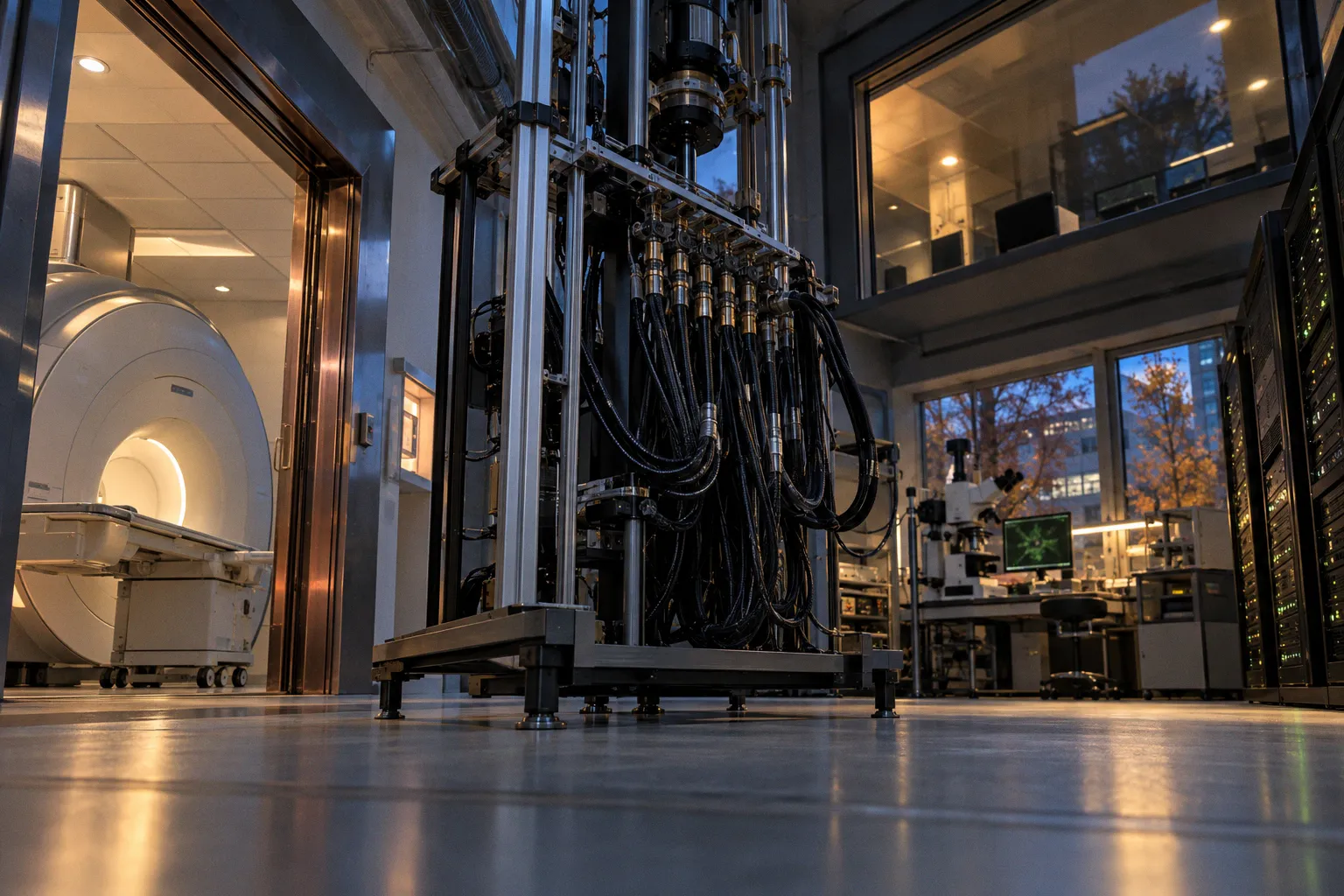
The exact result depends on the scanner, gradient set, sequence timing, acoustic enclosure, measurement position, and the way the sound is weighted. There is no single “3T noise level” that describes every installation.
The engineering cause is less ambiguous. Gradient coils vibrate because rapidly changing currents interact with the static magnetic field. Every readout line, phase-encode step, and diffusion-encoding moment changes the electromagnetic forces acting on the gradient assembly. Those forces become structural vibration, and structural vibration becomes sound.
The consequence, when it is not characterized, is familiar: a patient moves, hearing protection is poorly fitted, a scan is interrupted, or an otherwise usable protocol produces images that cannot be interpreted.
The Physics of Lorentz Forces: Why Gradient Coils Vibrate
The static magnetic field does not, by itself, generate the familiar clicking and banging of an MRI scan. The acoustic event begins when current flows through a conductor in the presence of the main field and changes with time. The resulting Lorentz force acts on the gradient conductors. The force is transferred through the coil former, support structures, cryostat, and bore enclosure, where some of the mechanical energy is radiated as sound.
A simplified expression is useful:
\[
\mathbf{F} = \mathbf{J} \times \mathbf{B}_0
\]
Here, the current density in the gradient conductor interacts with the static field \(B_0\). In a real scanner, the geometry is more complicated than the equation suggests. The force distribution depends on conductor layout, shielding, mechanical constraints, pulse shape, amplifier behavior, and the way the gradient assembly is mounted. But the practical implication is clear: faster and larger current changes can create stronger mechanical excitation, while the structure determines which parts of that excitation become audible.
Field strength matters, but not in the simplistic sense that a higher \(B_0\) automatically requires a stronger gradient for the same k-space trajectory. The required gradient amplitude is determined primarily by the desired spatial encoding, field of view, resolution, bandwidth, timing, and trajectory. A given k-space path does not become intrinsically more demanding merely because the main field has increased from 3T to 7T.
Higher field does change the engineering environment around that trajectory. Gradient hardware, bore geometry, sequence timing, peripheral nerve stimulation limits, susceptibility effects, RF constraints, and available performance margins may all change. A 7T system may use different gradient hardware or operate with different timing and encoding choices from a 3T system. Those system-level differences can produce a different acoustic signature, but they should not be reduced to a universal rule that \(B_0\) alone raises the gradient requirement.
The vibration also has a frequency spectrum rather than a single pitch. Gradient switching creates periodic and transient forces. Some components of those forces couple efficiently into structural modes of the gradient assembly; others are attenuated by the mechanical design. When the temporal content of a sequence approaches a strong mechanical mode, the assembly can respond more vigorously. The effect is system-specific and sequence-specific. It is one reason that two protocols with similar nominal gradient amplitudes can sound noticeably different.
A fast EPI sequence often sounds different from a conventional spin-echo acquisition because its gradient trains contain rapid, repeated switching and long echo trains. In some scanner and sequence combinations, one or more prominent spectral components may fall near a mechanical resonance. In others, the dominant sound may be governed by a different mode, a different harmonic, or the interaction between the gradient waveform and the structure. Resonance is therefore a useful mechanism to investigate, not a universal explanation for every EPI sound.
The mechanical assembly constrains the mitigation options. Additional damping can reduce ringing, but it may also reduce gradient efficiency or increase the time needed to reach and settle at a target amplitude. A stiffer structure can move a resonance away from an important operating band, while changing mass and stiffness elsewhere in the system. Vacuum isolation, acoustic barriers, constrained-layer damping, and improved mechanical coupling can all help, but each introduces packaging, thermal, service, or bore-space constraints.
That trade-off is why acoustic noise reduction in high field MRI cannot be treated as a cosmetic hardware project. The sound is an output of the same electromechanical system that determines gradient performance, scan time, image distortion, and patient access.
Quantifying the Soundscape: From 3T Clinical Standards to 7T Extremes
The first mistake in an acoustic assessment is to ask for one number and treat it as a property of the scanner. A meaningful measurement needs a defined sequence, gradient mode, patient position, microphone location, frequency weighting, averaging method, and peak-versus-equivalent-level convention.
A routine gradient-echo sequence, a diffusion EPI acquisition, and a long turbo spin-echo train do not load the gradient assembly in the same way. Even within one sequence family, acceleration, partial Fourier, echo spacing, bandwidth, resolution, and gradient duty cycle can change the sound field.
Typical clinical systems can produce sound in the broad range of roughly 80–110 dB for less aggressive acquisitions, while EPI, diffusion, and long echo-train sequences may be substantially louder. Measurements near 130 dB have been reported for particular high-demand readouts and measurement locations, but that value should not be presented as a universal output of a 3T scanner. A measurement at the bore axis is not automatically the same as the exposure at the patient’s ear, and peak SPL is not interchangeable with an A-weighted time-average level.
At 7T, acoustic output can be higher for some protocols, but the increase is not a simple field-strength conversion. The scanner’s gradient design, sequence implementation, bore acoustics, and operating constraints all contribute. Comparative studies of 3T and 7T brain or inner-ear protocols have reported materially higher average and peak levels at 7T in selected conditions. Those findings are clinically useful, but they describe the tested systems and sequences rather than establishing a universal 7T penalty.
A practical comparison looks like this:
| Sequence class | Typical acoustic tendency | Main mechanical driver | What must be measured |
|---|---|---|---|
| Routine GRE or SE | Often lower than long echo-train or diffusion protocols, but still system-dependent | Moderate gradient switching and repeated readout events | Time-averaged level and dominant spectral bands |
| EPI and diffusion | Frequently among the louder clinical acquisitions | Rapid readout switching, high duty cycle, and repeated polarity reversals within the echo train | Peak level, echo-train spectrum, and patient-ear exposure |
| TSE or FLAIR | Can be loud because of long echo trains and repeated refocusing events | Repeated gradient activity over a prolonged acquisition | Exposure duration as well as maximum level |
| Inner-ear or temporal-bone imaging | May combine high bandwidth, fine resolution, and demanding encoding | High-performance readouts and sequence-specific gradient timing | Spatial variation across the patient position and frequency content |
The regulatory framework should also be handled with care. MRI sites operate under applicable national regulations, professional guidance, manufacturer specifications, and local safety procedures. Limits may distinguish between peak and time-averaged exposure, use different frequency weightings, or specify how hearing protection and acoustic output are to be evaluated. A scanner is not automatically compliant because one number in a vendor document is below another number in a safety standard.
The same caution applies to dB(A) and dB SPL. A-weighting reduces the contribution of frequencies to approximate human hearing sensitivity under a defined convention. Unweighted SPL describes sound pressure without that correction. Peak SPL, RMS SPL, equivalent continuous level, and frequency-weighted exposure answer different questions. Comparing them as if they were interchangeable can produce a technically neat but clinically meaningless risk assessment.
For a protocol review, the useful record includes:
- the exact scanner and gradient configuration;
- the sequence version and all relevant acceleration or timing settings;
- the microphone position or dosimetry method;
- peak, average, and frequency-weighted values;
- the duration of each loud segment;
- the hearing protection used and its fit;
- whether the measurement was made with a patient, phantom, head coil, or empty bore.
The scanner does not have one acoustic signature. The protocol, hardware, measurement position, and protection system create the exposure together.
Clinical Risks: Hearing Threshold Shifts and Patient Compliance
MRI acoustic risk is not determined by a single threshold at which every patient experiences the same outcome. Exposure depends on level, duration, spectrum, individual susceptibility, hearing protection, and the quality of the fit. A short, high-level event and a longer exposure at a lower level can create different risks even when a simple meter reading appears similar.
Very loud gradient noise can produce temporary auditory symptoms, including a sensation of muffled hearing or tinnitus. Whether those symptoms occur depends on the actual exposure and the protection available. They should not be predicted with a universal incidence or a fixed time-to-onset claim. Permanent injury is a more serious possibility associated with excessive exposure, but it cannot be inferred from the nominal field strength or from the sequence name alone.
This is where measurement matters. If the protocol is close to a site’s permissible exposure boundary, the team needs an exposure assessment rather than an assumption that standard earplugs provide a fixed amount of attenuation. Real-world attenuation varies with insertion, seal, anatomy, motion, and frequency. Manufacturer ratings are obtained under specified test conditions and do not necessarily equal the protection achieved by a patient inside a scanner.
The clinical consequence is not limited to hearing. Acoustic load changes behavior. A patient may tense, press the emergency call button, start speaking, or move during the loudest part of the sequence. That motion is particularly damaging in diffusion-weighted imaging, where the measurement is sensitive to displacement, eddy-current effects, susceptibility, and phase inconsistencies. A scan can be technically within its acoustic limit and still fail because the patient cannot tolerate the experience.
The relationship with anxiety and sedation is similarly conditional. Children, patients with sensory sensitivities, people with pre-existing hearing concerns, and patients undergoing long or unfamiliar examinations may need a more deliberate acoustic strategy. Lower noise can improve cooperation, but sedation decisions are influenced by age, diagnosis, preparation, anxiety, scan duration, and institutional practice. Acoustic exposure is one factor, not a universal direct predictor of sedation.
That distinction matters in pediatric imaging. A quieter protocol may reduce distress and motion, but it does not remove the need for communication, rehearsal, appropriate immobilization, and a protection system that fits the child. A hearing-protection device that works for an adult may leak around a smaller ear or interfere with a head coil. The solution must be tested in the actual workflow, not selected from an attenuation figure alone.
A failed scan also has an engineering cost. Repeating a diffusion series extends the examination, increases the patient’s time in the bore, and may require repeating loud gradient activity. The second attempt is not guaranteed to succeed if the team has not identified the source of the first failure. In practice, acoustic characterization belongs in protocol development alongside distortion checks, SAR review, peripheral nerve stimulation assessment, and motion robustness.
Algorithmic Noise Reduction: Reshaping Gradient Waveforms
Hardware changes to the gradient assembly can be effective, but they are difficult to apply across an installed base. Damping layers, modified mounts, structural reinforcement, acoustic barriers, and changes to the gradient package may require a major service intervention. Some interventions can be performed with the magnet cold; others may be possible without a full cold-cycle. The requirement depends on the hardware, the vendor, the service procedure, and the location of the component being changed.
That variability is one reason sequence-based mitigation is attractive. It can sometimes reduce noise without rebuilding the scanner, provided the new waveform preserves the requirements that matter for the image. A quieter sequence is not a success if it changes diffusion weighting, echo time, readout bandwidth, refocusing behavior, geometric distortion, or contrast in a way the clinical application cannot accept.
Waveform optimization usually begins by examining the gradient demand in time rather than treating the nominal amplitude and slew rate as independent settings. A trapezoidal lobe may be replaced or modified with a smoother profile. The same k-space area can be distributed over a longer interval, reducing abrupt current changes and changing the spectral content of the mechanical excitation. The result may move energy away from a strong structural mode rather than simply making every part of the waveform smaller.
Sinusoidal or pre-emphasized profiles are not automatically quieter. Their value depends on the scanner’s transfer function, the mechanical resonances of the gradient assembly, and the sequence timing. A profile that avoids one resonance may excite another. The correct process is to measure the response, model or characterize the relevant spectral bands, then validate the modified sequence for image quality and scan time.
Published sequence-specific studies have reported reductions on the order of several decibels, including substantial reductions for optimized TSE and GRE implementations under controlled conditions. Results such as approximately 14 dB(A) for some TSE approaches or approximately 17 dB(A) for some GRE approaches should be read as examples of what a particular optimization achieved, not as guaranteed reductions for every scanner. The acoustic benefit depends on the original waveform, the hardware, the measurement method, and whether the sequence can tolerate a longer readout.
The principal trade-off is time. Spreading gradient area across a longer interval can lengthen the readout or the echo spacing. In EPI, that may increase geometric distortion, T2* blurring, or sensitivity to off-resonance. A lower slew rate may also alter the minimum achievable echo time or the spacing between echoes. In diffusion imaging, the same change can affect the diffusion preparation and the total echo time, which may reduce signal even when the nominal b-value is preserved.
EPI polarity, resonance, and spectral shaping
EPI deserves a more precise description because its acoustic behavior is often explained too loosely. In a conventional EPI echo train, the readout gradient reverses polarity between successive echoes so that adjacent lines of k-space are traversed in alternating directions. The phase-encoding blips advance the trajectory from one line to the next. This alternating readout occurs within the echo train, not simply between separate shots.
Changing the timing, shape, or ordering of those gradient events can change the spectrum of the mechanical excitation. In some implementations, a modified polarity pattern or trajectory arrangement can move prominent spectral components away from a strong structural resonance. In others, the same intervention may have little benefit or may create a new peak. It must be evaluated on the target hardware.
The image trajectory also has to remain correct. Any change in gradient timing requires corresponding trajectory calibration, accounting for gradient delays, eddy currents, concomitant-field effects where relevant, and reconstruction assumptions. A visually quieter scan that uses an inaccurate trajectory is not a successful noise-reduction strategy.
Pre-emphasis is another useful lever, although it is not a universal noise suppressor. Gradient pre-emphasis is normally used to compensate for predictable system responses such as eddy-current-induced distortions and delays. Better compensation can reduce unwanted departures from the commanded waveform and may lessen mechanical excitation in some systems. It can also increase fidelity to a demanding waveform without extending the sequence. The acoustic result depends on the entire electromechanical chain and should be measured rather than assumed.
A responsible optimization therefore has two parallel acceptance criteria:
1. The image must retain the intended contrast, resolution, encoding, diffusion weighting, distortion performance, and artifact behavior.
2. The acoustic exposure must improve at the patient position under the exact operating conditions used clinically.
If one side is missing, the protocol has been optimized only on paper.
Integrated Mitigation: Combining Passive Insulation with Active Noise Control
No single intervention reliably solves the acoustic problem across all high-field examinations. Gradient design determines the source. Sequence timing determines how the source is driven. Bore construction and room treatment determine how much sound reaches the patient. Hearing protection determines how much reaches the ear. Patient preparation determines whether the person can remain still despite what remains.
Passive protection is still the first line of defense. MRI-compatible earplugs can provide useful attenuation when correctly fitted. Earmuffs, passive headphones, and combinations of plugs and muffs can add protection, but their performance depends on seal, compatibility with the head coil, comfort, and the frequency spectrum of the scanner noise. The attenuation number printed on a package is not a patient-specific measurement.
Headphones are not universally incompatible with high-density receive arrays. MRI-compatible headphones and transducers can be designed for use with receive coils, provided they meet the scanner’s safety and compatibility requirements. The practical constraints are real: the device may alter coil positioning, create pressure points, interfere with immobilization, or introduce susceptibility or RF concerns. Those are design and integration problems, not a categorical impossibility.
Acoustic insulation in 3T MRI suites can reduce room radiation and reflected sound, but it cannot eliminate vibration generated inside the gradient assembly. The bore liner, enclosure, room panels, ventilation paths, door seals, and structural connections all influence what reaches the patient and the operator. A room that sounds quieter outside the magnet may still expose the patient to a strong near-field sound field.
Active noise control adds another layer. An ANC system measures the acoustic field or a reference signal and drives a counter-signal through a compatible transducer. Cancellation is most effective where the system has a stable relationship between the reference, the control source, and the error sensor. It is not equally effective across all frequencies or positions.
In the bore, geometry makes the problem difficult. The sound field is not necessarily uniform around the head, and the patient’s position can change the relationship between the gradient source and the ear. Low-frequency components are often easier to control because the controller has more time within each acoustic cycle and the wavelength is longer. Higher-frequency components demand shorter latency, accurate phase control, and transducers that can operate safely in the MRI environment. The useful bandwidth is therefore system-specific.
Pneumatic systems can keep electrically active components farther from the magnet, but the tubing, transducer response, and propagation delay limit the achievable cancellation. Electromechanical systems can provide more direct control, while creating their own requirements for non-ferromagnetic construction, RF compatibility, susceptibility management, and mechanical integration. Neither architecture should be treated as automatically superior.
The practical deployment questions are straightforward, even if the answers are not:
- Is the system integrated with the scanner, installed as a bore insert, or supplied as an external accessory?
- Has attenuation been measured at the patient’s ears rather than inferred from a laboratory specification?
- Does the system remain effective during the actual sequence, including its loudest transients?
- Does it interfere with the receive array, positioning, monitoring, emergency access, or communication?
- Is the control system stable when the patient’s head position and anatomy vary?
- Has the protection been validated for the complete protocol rather than for a short test waveform?
Acoustic compliance is a stack, not a switch: passive attenuation, waveform optimization, room treatment, and active control cover different parts of the problem.
The Engineer’s Burden
Acoustic noise in MRI is a physics constraint, but the clinical failure is usually a systems failure. The Lorentz force explains the source. The gradient assembly determines how that force becomes vibration. The sequence determines which frequencies are driven and for how long. The room and protection system determine the exposure that reaches the patient.
A protocol near an applicable exposure limit requires measurement, not reassurance. A 7T diffusion sequence should not rely on earplugs alone without checking the actual attenuation and patient fit. A TSE or EPI protocol should not be assumed to be quiet because its nominal gradient amplitude looks ordinary. An ANC system should not be treated as a black box when its performance depends on frequency, position, latency, and integration with the receive array.
The best mitigation strategy is layered:
- characterize the acoustic spectrum of the exact sequence on the exact scanner;
- identify the dominant mechanical bands and transient events;
- reshape gradient waveforms where image timing allows it;
- validate the EPI trajectory and contrast after any timing change;
- use hearing protection that fits the patient and the coil geometry;
- add passive room or bore treatment where it addresses the relevant transmission path;
- use active control only after its actual bandwidth and attenuation have been measured;
- repeat the assessment after software, hardware, coil, or protocol changes.
The goal is not to make every scan silent. That is neither realistic nor necessary. The goal is to keep exposure within the applicable safety framework while preserving the image quality and workflow that justified the examination in the first place.
A failed scan is often the first visible sign that the acoustic design was incomplete. The quieter and safer protocol is the one that has been measured at the patient position, tested with the intended receive array, checked for image consequences, and designed around the specific mechanical behavior of the scanner rather than around a generic field-strength label.