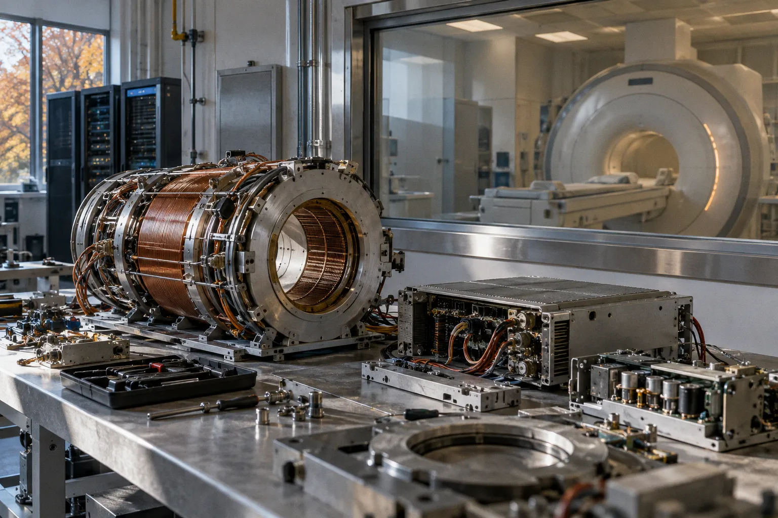
It is also sufficient to turn the scanner’s conductive surroundings into secondary electromagnetic components.
Those components do not follow the commanded waveform. They oppose it, delay it, and continue to evolve after the gradient current has returned to zero. The result is not merely electrical inefficiency. The actual magnetic field seen by the spins diverges from the field assumed by the pulse sequence. Spatial encoding degrades. Phase accumulates along the wrong trajectory. The reconstruction receives k-space data generated by a gradient system that did not produce the nominal gradient waveform.
This is the central problem addressed by gradient coil eddy current compensation techniques. Active shielding, pre-emphasis, calibration, sequence design, and post-processing do not remove the underlying electromagnetic physics. They constrain its consequences.
The physics of induced currents in MRI hardware
The mechanism begins with Faraday’s law. A changing magnetic flux induces an electromotive force in any conductive structure intersecting that changing field. In an MRI system, those structures are not limited to the gradient conductors themselves. They include the cryostat, cryoshields, RF shields, conductive support structures, coil housings, and sometimes components inside the receive array.
A rapidly changing gradient field therefore creates circulating currents outside the intended gradient coil. These are eddy currents. Their direction opposes the change that produced them, consistent with Lenz’s law. Their amplitude depends on the rate of flux change, the geometry of the conductive loop, the material conductivity, and the effective resistance and inductance of the structure.
The relevant sequence parameter is not only gradient amplitude. Slew rate matters. A modest gradient switched aggressively can induce more problematic behavior than a larger gradient ramped slowly. The derivative of the field is the trigger.
The induced current generates its own magnetic field. That field is spatially distributed and temporally delayed. It may have a component aligned with the commanded gradient, a component that behaves like a residual offset, and cross-axis components that couple into the other gradient directions. The scanner therefore operates with several superimposed fields:
- the nominal gradient field commanded by the sequence;
- the delayed and opposing fields generated by conductive structures;
- static-field perturbations associated with heating and mechanical interaction;
- residual spatial terms that are not represented by the ideal linear gradient model.
The resulting gradient response is often described by a sum of exponential components. Each conductive structure behaves as an electromagnetic compartment with its own effective amplitude and time constant. One component may decay rapidly. Another may persist substantially longer. A useful abstraction is:
\(G_{\text{actual}}(t) = G_{\text{commanded}}(t) + \sum_i A_i e^{-t/\tau_i}\)
The equation is simplified. Real systems include spatial dependence, cross terms, nonlinearities, amplifier dynamics, and coupled hardware responses. But the engineering implication is direct: one correction constant is insufficient when several conductive structures contribute distinct decay behavior.
Why EPI exposes the problem
Echo-planar imaging is especially sensitive because it switches gradients rapidly while traversing k-space with alternating readout polarity. The readout trajectory depends on precise timing. A small phase discrepancy between adjacent echoes shifts the effective sampling positions.
Eddy-current-induced phase errors contribute directly to Nyquist N/2 ghosting. The ghost is not an arbitrary reconstruction defect. It reflects a mismatch between the assumed and actual k-space trajectory. If the positive and negative readout lobes are not equivalent after the conductive environment responds, the even and odd echoes carry different phase errors. The image reconstruction interprets those errors as spatial displacement.
The damage is more severe when several conditions coincide:
- high slew rate;
- long echo trains;
- strong diffusion gradients;
- oblique imaging orientations;
- short echo spacing;
- large field of view combined with demanding spatial encoding;
- low SNR, where residual ghosts approach the intensity of real anatomy.
In diffusion EPI, the problem is compounded by the large gradient moments used to encode motion at the microscopic scale. The sequence is deliberately sensitive to phase. Eddy currents exploit that sensitivity.
The image may show geometric distortion, signal pile-up, signal loss, ghosting, or direction-dependent misregistration. These manifestations are often grouped under gradient-related artifacts, but they have different physical causes. A gradient delay, an eddy-current field, gradient nonlinearity, B0 inhomogeneity, and subject motion can coexist in the same acquisition. Treating them as one correction problem produces unstable results.
The reconstruction cannot repair a k-space trajectory that the hardware never generated unless the deviation is measured, modeled, and supplied to the correction process.
Active shielding: engineering the primary defense
Active shielding in MRI gradient coils reduces the magnetic field that extends beyond the intended imaging region. A conventional gradient coil generates a field not only inside the bore but also outside the primary winding geometry. That external field changes magnetic flux through the cryostat and other conductive structures. More flux change means larger induced currents.
An actively shielded gradient assembly adds secondary conductors designed to oppose the external field of the primary gradient coil. The goal is not to cancel the imaging gradient inside the usable volume. The goal is to suppress the field outside the gradient assembly while preserving the required spatial derivative near the patient.
The design is a constrained field-shaping problem. The primary and shield windings must satisfy several conditions simultaneously:
- generate the required linear gradient within the imaging volume;
- preserve gradient efficiency;
- limit external fringe fields;
- tolerate the electrical current required for the target amplitude and slew rate;
- manage Lorentz forces and acoustic vibration;
- fit within the available bore and mechanical envelope;
- avoid unacceptable inductance and amplifier burden.
Active shielding became widely adopted in clinical systems in the mid-1990s. Modern actively shielded gradients can reduce unwanted eddy-current fields to approximately the percent level or below, depending on the system, spatial location, gradient axis, operating condition, and measurement method.
That number should not be misread. Percent-level residual behavior is still enough to damage phase-sensitive imaging. A one-percent field error applied to a strong diffusion gradient is not equivalent to a one-percent error in a low-demand localizer. The image consequence depends on the gradient moment, echo timing, k-space ordering, and the tissue signal being measured.
Shield design does not create a closed electromagnetic system
The primary gradient coil and its shield remain coupled. The shield carries high currents. It has its own inductance, resistance, mechanical forces, and frequency response. The field cancellation is therefore imperfect and frequency-dependent.
At one switching pattern, the shield may suppress the dominant external field effectively. At another, the timing and spatial distribution of induced currents can produce residual components that are not captured by a simple scalar correction. The correction must tolerate:
- multiple decay constants;
- axis-to-axis coupling;
- gradient waveform asymmetry;
- thermal drift;
- loading changes;
- amplifier response;
- installation-specific conductive structures.
The cryostat remains a particularly important source of induced current. Even with active shielding, the time-varying field can couple into conductive layers. Those currents dissipate power as Joule heating. The thermal consequence is not always visible in a single image, but it can affect static-field stability and cryogen boil-off in superconducting systems.
The gradient system is therefore not only an imaging actuator. It is an electromagnetic heating source embedded in a complex conductive environment.
Mechanical interaction with the static field
The static field, \(B_0\), interacts with the magnetic moments generated by induced currents. If the induced-current field is misaligned with the main field, the conductive structure can experience force and torque. The effect is relevant to both scanner hardware and conductive implants.
The same rapidly switched gradient that perturbs the k-space trajectory can generate mechanical stress, vibration, and acoustic noise. These are not independent nuisances. They originate in the same Lorentz-force environment. A gradient design that increases current and slew rate must also manage mechanical reaction forces, conductor support, vibration modes, and patient acoustic exposure.
High-performance gradient hardware design is therefore bounded by several coupled limits. Electrical performance alone is an incomplete specification.
Pre-emphasis calibration and waveform modification
Before active shielding became common, gradient pre-emphasis was the primary method for compensating eddy-current effects. The method remains necessary because active shielding does not eliminate all induced currents.
Pre-emphasis does not reduce the physical eddy currents inside the cryostat or surrounding conductive structures. It modifies the commanded gradient current so that the magnetic field remaining after the induced fields are superimposed more closely matches the intended waveform.
The command is deliberately distorted to make the resulting field less distorted.
If the conductive environment creates a delayed opposing field after a gradient transition, the amplifier can receive a compensating waveform with additional components timed to counter that response. The pre-emphasis filter may include several amplitudes and time constants. In practical systems, those coefficients are proprietary and vary with gradient axis, hardware configuration, field strength, operating state, and calibration procedure.
The conceptual operation is:
1. Define the target gradient waveform.
2. Characterize the system’s actual response.
3. Estimate the induced-current components.
4. Calculate a compensating input waveform.
5. Apply that waveform through the gradient amplifier.
6. Measure the residual error.
7. Update the compensation parameters.
The process is inverse system identification. The scanner is treated as a dynamic system with a measurable impulse response. The compensation filter is designed to invert the relevant part of that response without destabilizing the amplifier or exceeding hardware limits.
The response is multi-exponential, not instantaneous
Eddy-current compensation becomes difficult because different structures respond on different time scales. A fast component may affect the edge of a gradient ramp. A slower component may produce a residual field through the echo train. The compensation waveform must address both without introducing an opposite error.
The scanner must also distinguish between:
- direct gradient amplifier dynamics;
- primary-coil inductance;
- shield-coil response;
- eddy-current fields in the cryostat;
- cross-axis coupling;
- gradient nonlinearity;
- temporal drift.
These effects can overlap in the measured response. A calibration model that assigns every deviation to eddy currents will compensate the wrong mechanism.
The most useful calibration is not the one that produces the cleanest response in a single test waveform. It is the one that remains stable across the waveform families used clinically. A correction tuned to a short trapezoid may not perform identically for a diffusion lobe, an EPI readout train, or a non-Cartesian trajectory.
What calibration actually measures
Gradient calibration can use field probes, imaging-based measurements, NMR phase methods, or combinations of hardware and sequence diagnostics. The objective is to estimate the actual field as a function of time and position.
A phase-based measurement is especially informative because gradient errors accumulate into phase. If a known spin population experiences a gradient waveform, the resulting phase evolution contains information about the time-integrated field. The measurement can expose delayed responses that are difficult to infer from amplifier current alone.
A useful calibration must consider:
- gradient amplitude;
- ramp timing;
- polarity;
- duty cycle;
- axis orientation;
- waveform repetition;
- thermal state;
- physical location within the imaging volume.
The final correction may be represented as a digital pre-emphasis impulse-response filter. The filter coefficients are applied before the nominal waveform reaches the gradient amplifier. In some systems, additional sequence-level corrections are applied after acquisition. The hardware and reconstruction layers are therefore linked.
Where the residual error appears in the image
The imaging consequence depends on how the gradient error enters the acquisition. The same physical eddy-current field can produce different artifacts in different sequences.
EPI and Nyquist ghosting
In EPI, the readout gradient alternates polarity. Eddy-current response does not necessarily reverse with the same symmetry. The positive and negative readout lobes can therefore experience different amplitude and phase histories.
The reconstruction commonly separates even and odd echoes. If their phase relationship is wrong, the signal is displaced by half the field of view in the phase-encoding direction. This is the characteristic Nyquist N/2 ghost.
Ghost correction often estimates a phase difference between echo parity classes and applies a correction during reconstruction. That can reduce the visible artifact. It does not prove that the gradient hardware is correctly generating the intended trajectory. A residual phase correction may hide a systematic hardware error while leaving spatially varying or direction-dependent distortions unresolved.
Diffusion imaging
Diffusion weighting magnifies the effect of gradient imperfections because the sequence uses strong, carefully timed gradient moments. Eddy-current fields generated by those moments can produce shearing, scaling, and spatial displacement of diffusion-weighted volumes.
The distortion is direction-dependent. Each diffusion gradient orientation excites a different electromagnetic response in the scanner hardware and a different interaction with B0 and the subject. The resulting volumes can be misaligned even when the structural image appears acceptable.
Typical correction pipelines may estimate volume-to-volume transformations, often using affine registration and susceptibility correction. These methods are useful. They are not a substitute for hardware calibration. Registration can align image features after acquisition, but it cannot recover signal lost through severe intravoxel dephasing or reconstruct k-space samples that were never acquired at the assumed positions.
Non-Cartesian trajectories
Spiral, radial, and other non-Cartesian acquisitions are particularly dependent on trajectory accuracy. The reconstruction assumes a continuous path through k-space. A delayed or spatially distorted gradient changes that path.
A trajectory error can produce blurring, ringing, geometric distortion, and signal loss. The reconstruction may use a measured trajectory rather than a nominal one. This improves fidelity, but only if the trajectory measurement represents the actual operating state. Thermal drift, gradient loading, and sequence-specific waveform history can change the response.
Gradient nonlinearity is related but distinct
Gradient nonlinearity correction methods address the spatial deviation of the gradient field from an ideal linear field. Eddy-current compensation addresses temporal and induced-field behavior. The two can interact, but they should not be collapsed into one correction.
Gradient nonlinearity causes spatially dependent scaling and geometric distortion. Eddy currents cause time-dependent field errors and phase deviations. A scanner can have good geometric linearity and poor temporal fidelity. It can also have well-compensated temporal response but significant peripheral spatial nonlinearity.
A complete correction chain may need to account for both:
| Error source | Primary mechanism | Typical consequence | Main correction layer |
|---|---|---|---|
| Eddy currents | Induced fields in conductive structures | Phase error, ghosting, delayed gradient response | Active shielding, pre-emphasis, trajectory correction |
| Gradient nonlinearity | Spatially nonideal gradient field | Geometric distortion, location-dependent scaling | Spatial field-model correction |
| B0 inhomogeneity | Static-field variation | Off-resonance distortion, signal pile-up | Shimming, field mapping, reconstruction correction |
| Gradient delay | Timing mismatch in gradient response | Shifted k-space trajectory, blurring | Hardware calibration, measured trajectory |
| Motion | Subject displacement and phase change | Misregistration, ghosting, signal loss | Prospective or retrospective motion correction |
The table is not a substitute for a system model. It is a reminder that artifact labels are not physical diagnoses.
Pre-emphasis is not a cancellation of current. It is a cancellation of the field error produced by current.
Compensation at the hardware and sequence layers
The strongest systems use several layers of mitigation. No single method covers every residual.
Electrical pre-emphasis
The digital gradient command is modified before amplification. The correction targets the measured impulse response of each gradient axis. Multi-exponential models are common because the surrounding conductive structures do not share one time constant.
The filter must remain bounded. An aggressive inverse response can demand amplifier behavior that exceeds voltage, current, or slew constraints. A correction that is mathematically exact for one narrow waveform can be unusable across the full sequence library.
The practical objective is not zero error under ideal conditions. It is low residual error across clinically relevant waveforms and thermal states.
Active shielding
The shield reduces the external magnetic field that drives induced currents in the first place. It lowers the burden placed on pre-emphasis and reduces coupling into the cryostat. The shield must preserve useful gradient efficiency while limiting fringe fields and mechanical stress.
A shield that is electrically effective but mechanically unstable is not a successful design. Vibration can contaminate functional imaging and increase acoustic output. A shield that imposes excessive inductive burden can constrain amplifier performance. Hardware architecture is a compromise constrained by Maxwell’s equations and by the mechanical envelope.
Coil and structure design
Conductive structures can be segmented or slotted to interrupt large current loops. Electrical isolation and geometry reduce the area available for circulating currents. This approach is used in relevant coil and shield components, but it introduces its own design constraints.
Slots can alter mechanical stiffness, thermal conduction, RF behavior, manufacturability, and field uniformity. The best layout minimizes induced-current pathways without creating new resonances or unacceptable local field errors.
RF shields are particularly sensitive because they must maintain electromagnetic function at radiofrequency while limiting interaction with rapidly switched gradient fields. The hardware cannot be optimized for one frequency regime in isolation.
Sequence-level design
Pulse-sequence engineers can reduce susceptibility by controlling gradient transitions, echo spacing, gradient polarity, and waveform timing. This does not eliminate the hardware response. It changes the excitation pattern applied to the response.
The sequence can also use bipolar designs, reversed phase-encoding acquisitions, navigator information, or calibration scans to estimate residual errors. These methods consume time, signal, or reconstruction complexity. They are justified when the target measurement is more sensitive to phase than to scan efficiency.
Rapid MRI acquisition therefore has a cost beyond nominal temporal resolution. Every faster transition loads the gradient system and its conductive environment more aggressively.
Post-processing and measured trajectories
If the actual k-space trajectory is measured or modeled accurately, the reconstruction can compensate for some deviations. The correction may use a nonuniform reconstruction, phase correction, volume registration, or a field-based model.
The limitation is information. A post-processing algorithm can correct a known and sufficiently sampled error. It cannot infer an unmeasured trajectory with arbitrary precision from a damaged image. It cannot restore signal that was dephased inside a voxel. It cannot distinguish hardware-induced phase from motion or B0 variation without additional constraints.
The reconstruction layer should therefore receive hardware characterization, not merely a generic artifact label.
Stability, heating, and long acquisitions
Eddy currents are often discussed as an image-quality problem. They are also a system-stability problem.
The induced currents dissipate energy through Joule heating. In the cryostat and other conductive structures, this can perturb thermal conditions. In superconducting systems, heating can influence static-field stability and cryogen boil-off. The magnitude depends on gradient duty cycle, waveform content, conductive geometry, shielding, and operating state.
This matters for long functional runs, diffusion protocols, high-resolution EPI, and repeated high-duty-cycle acquisitions. A calibration performed at one thermal state may not perfectly represent the system later in the examination. The resulting drift can appear as temporal instability, registration error, or changing artifact severity.
The scanner is not a static transfer function. Its response can evolve under load.
That fact constrains claims about nominal gradient performance. A headline gradient amplitude or slew rate does not fully describe acquisition capability. The useful specification includes:
- temporal fidelity under realistic duty cycle;
- residual eddy-current field;
- cross-axis coupling;
- stability during sustained operation;
- acoustic and mechanical behavior;
- trajectory accuracy;
- calibration repeatability;
- correction behavior across sequence families.
A system that reaches an aggressive nominal waveform but produces unstable k-space sampling is not delivering equivalent performance.
Advanced mitigation for high-speed and ultra-high-field systems
Ultra-high-field MRI increases the value of precise acquisition control. B0 inhomogeneity, susceptibility effects, RF constraints, and distortion already make the experiment difficult. Residual gradient errors add another layer of phase and geometric instability.
High-speed sequences intensify the problem through rapid switching and dense k-space traversal. The hardware must tolerate the induced electromagnetic response while maintaining a field waveform that the reconstruction can trust.
Several strategies become more important as performance demands rise:
1. Field-based gradient monitoring. Directly measure the generated field rather than relying only on commanded current. This exposes amplifier delays, eddy-current tails, and cross-axis terms.
2. Sequence-specific trajectory calibration. Characterize the waveform family actually used by the acquisition. A generic system response is useful, but not always sufficient for spiral, diffusion, or long EPI trains.
3. Multi-axis response modeling. Include cross terms when the induced field from one gradient axis contributes to another. Oblique imaging makes this especially relevant.
4. Thermal-state tracking. Repeat or update calibration when sustained gradient duty cycle changes the hardware state. Static coefficients are less reliable under heavy loading.
5. Integrated reconstruction models. Propagate measured gradient behavior into the k-space reconstruction rather than treating it only as a final image-space artifact.
6. Hardware-aware sequence optimization. Penalize waveforms that generate large residual tails, unnecessary current reversals, or high conductive loading when the resulting temporal resolution does not justify the cost.
These methods are not interchangeable. Field monitoring improves observability. Pre-emphasis improves the command. Active shielding reduces excitation of the conductive environment. Reconstruction correction accounts for residual error. Each operates at a different point in the chain.
How to evaluate gradient coil eddy current compensation techniques
A credible evaluation should not stop at a single phantom image or a manufacturer’s nominal gradient specification. The relevant question is whether the actual field response remains close to the intended response under the waveform conditions that matter.
A technical assessment should examine:
- residual gradient field after a rapid transition;
- decay behavior across multiple time constants;
- phase error in EPI;
- Nyquist ghost amplitude and spatial variation;
- diffusion-volume distortion across gradient directions;
- measured versus nominal k-space trajectory;
- cross-axis response during oblique imaging;
- stability after sustained high-duty-cycle operation;
- dependence on gradient polarity and waveform history;
- performance at the center and periphery of the imaging volume.
SNR is necessary but insufficient. A system may preserve average SNR while degrading spatial fidelity. Conversely, a correction can reduce ghost intensity while altering local phase in a way that affects quantitative diffusion or functional measurements.
The metric must match the application. For neuroimaging, the relevant output may be tractography stability, distortion consistency across directions, functional activation localization, or reproducibility of quantitative maps. For hardware development, the relevant output may be impulse-response fidelity, residual eddy-current amplitude, and thermal repeatability.
There is no single artifact score that captures all of these.
The boundary between compensation and concealment
Correction becomes misleading when it hides a hardware limitation without preserving the underlying measurement model. A reconstruction can make an image look cleaner while leaving quantitative values biased. This is particularly dangerous in diffusion imaging, spectroscopy, and functional studies where phase and spatial alignment carry scientific meaning.
A robust system should expose enough metadata to establish:
- which gradient waveform was commanded;
- which trajectory was measured or assumed;
- which pre-emphasis state was active;
- which gradient axes were calibrated;
- whether the correction was hardware-based or retrospective;
- whether thermal or load conditions differed from calibration.
Clinical users do not need raw impulse-response coefficients for every scan. Developers and researchers do need a defensible path from hardware behavior to reconstructed data.
The software layer cannot be separated cleanly from the acquisition layer. The image is the final output of both.
Conclusion
Gradient coil eddy currents are a direct consequence of fast magnetic-field switching inside a conductive machine. They induce opposing and lingering fields in cryoshields, RF shields, coil components, and other structures. Those fields alter the gradient waveform actually experienced by the spins.
Active shielding reduces the external flux that drives the problem. Pre-emphasis modifies the commanded current so the net field approaches the target waveform. Coil segmentation, structural design, sequence control, field monitoring, trajectory measurement, and post-processing address the residuals. None of them makes the underlying response disappear.
The correct engineering question is not whether a scanner has eddy currents. Every rapidly switched gradient system does. The question is whether the system measures, models, and constrains them well enough for the intended acquisition.
If the k-space trajectory is assumed rather than verified, high-performance gradient hardware remains partly nominal. The scanner may produce the requested waveform in software. The spins receive something else.