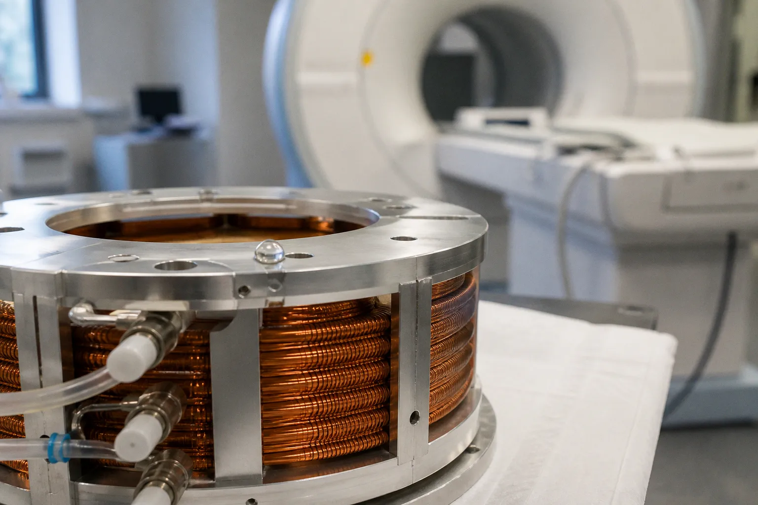
A demanding acquisition with many diffusion directions, high b-values, and long diffusion-encoding lobes asks the amplifiers and gradient coils to deliver substantial current repeatedly over an extended period. The exact current, voltage, slew rate, and duty cycle depend on the scanner, the gradient set, and the sequence implementation. There is no universal current draw for “a DTI scan.”
The underlying problem, however, is consistent across platforms: copper windings dissipate electrical energy as heat. That heat is removed by the scanner’s cooling system, but not instantaneously and not perfectly uniformly. As the gradient assembly, its housing, the bore liner, and nearby structures warm, the magnetic environment can change. The result may be a slow drift in B0, changes in spatial encoding, or a gradual loss of consistency between diffusion-weighted volumes.
This failure mode rarely announces itself with a dramatic system error. The scanner may pass daily QA. Eddy-current correction may be enabled. A phantom acquired under a short or modest-duty-cycle protocol may look entirely acceptable. The problem appears later, during the long acquisition that actually stresses the hardware. There may be no single universal point at which the data fail: the onset depends on the scanner’s thermal state, the sequence, the preceding workload, the room and cooling conditions, and the amount of recovery between scans.
That is what makes gradient coil heating diffusion MRI artifact so difficult to manage. It is not one artifact with one signature. It is a moving interaction between the gradient hardware, the magnetic field, the pulse sequence, and the reconstruction pipeline.
The Physics of Joule Heating in High-Performance Gradients
Modern clinical gradient systems are powerful instruments. A whole-body 3 T scanner may use gradient amplifiers capable of currents in the kiloampere range, with peak voltages of several thousand volts and slew rates that can reach hundreds of tesla per metre per second on high-performance systems. Gradient amplitudes vary considerably: standard clinical hardware and dedicated research systems do not share one universal specification.
Those headline numbers matter because resistive heating follows the familiar relationship \(P = I^2R\). If the current through a winding rises, the instantaneous power deposited as heat rises with the square of that current, assuming resistance is otherwise stable. The sequence does not need to operate continuously at its maximum rated amplitude to create a substantial thermal load. Repeated high-amplitude waveform segments, especially when separated by only brief periods of recovery, can produce a high average duty cycle.
The geometry of the gradient system adds another layer. A whole-body gradient coil must produce a controlled, spatially varying magnetic field over a large imaging volume. Increasing the volume that must be influenced is expensive in electromagnetic terms; the power and engineering demands do not scale in a simple linear way with bore size. This is one reason why a research gradient designed for particularly high amplitude or slew rate is not merely a standard clinical gradient with a larger number on the specification sheet.
Diffusion imaging is demanding because the gradients are not used as isolated, short events. Diffusion encoding typically relies on pairs of strong gradient lobes around the refocusing pulse. The duration and amplitude of those lobes depend on the desired b-value, diffusion time, available gradient strength, echo-time constraints, and sequence design. A high b-value may be achieved through different combinations of amplitude and duration, and those combinations do not impose identical thermal loads.
The same is true of direction count. A 60-direction protocol is not automatically more thermally demanding than every 30-direction protocol in a fixed proportion. The relevant variables include the number of volumes, the strength and duration of the diffusion gradients, the repetition structure, the sequence timing, and what the scanner has already acquired. The correct question is not simply how many directions appear in the protocol. It is how much gradient energy is deposited over time and how much opportunity the system has to remove it.
A useful distinction is between peak load and average load:
- Peak amplitude and slew rate determine how hard the amplifiers and coils are driven during individual waveform segments.
- Duty cycle determines how much of the acquisition is spent delivering that load rather than recovering from it.
- Sequence timing determines whether heat is deposited in tightly packed bursts or spread over a longer interval.
- Prior scans determine whether the system begins near a thermal steady state or with more available cooling margin.
- Recovery periods affect how much of the stored heat can leave the gradient assembly before the next run.
In a diffusion sequence, the gradient system may therefore spend a large fraction of the acquisition delivering energy to the coils. The cooling loop removes heat continuously, but the winding and surrounding structures have thermal mass. Temperature can continue to rise even while coolant is circulating and even during brief gaps in the waveform.
The gradient coil is the part of the scanner that does the real work — and it does that work by turning electrical power into heat.
The phrase “gradient coil heating diffusion MRI artifact” is useful only if it is understood as a systems problem. The heat does not need to damage the coil to damage the scan. A thermally safe acquisition can still be vulnerable to small field and geometric changes that matter to quantitative diffusion analysis.
Thermal Dynamics and the Mechanics of B0 Field Instability
The relevant question is not whether the coil gets hot. It does. The relevant question is where that heat goes, how quickly it moves through the scanner, and which magnetic properties change along the way.
The static B0 field in a superconducting MRI system is maintained and shaped by the main magnet and by a combination of passive and active shimming components. The gradient insert, bore liner, RF shield, passive shim structures, cryostat-related components, and other nearby materials do not all respond to heating in the same way. Their thermal expansion and magnetic susceptibility can change as temperature changes. Even a small change may matter when the sequence is sensitive to frequency, phase, or spatial registration.
Gradient coil temperature drift is therefore not identical to the temperature shown by a coolant sensor. The coolant temperature describes one part of the thermal system. The copper winding, coil former, epoxy, structural supports, shim components, and bore environment can have different temperatures and different time constants. A sensor may report that the cooling loop is within its expected operating range while the surrounding structure is still moving toward a new thermal equilibrium.
That lag is central to the problem. The heat produced in the winding is conducted outward gradually. Some of it is removed through active cooling; some is stored temporarily in the mass of the gradient insert and nearby components. The field response can continue to evolve after the most intense gradient activity has ended. Conversely, a system may begin a new scan with the coolant already close to its normal inlet temperature while other components remain warmer than they were at the start of the day.
The practical effect may include:
- a slowly changing resonance frequency or B0 offset;
- phase evolution across volumes acquired at different points in the run;
- changes in susceptibility-related distortion;
- gradual shifts in image geometry or registration quality;
- signal drift that is difficult to separate from physiological or scanner noise;
- altered consistency between b0 and diffusion-weighted images.
The magnitude and visibility of these effects are scanner- and protocol-dependent. Some systems provide field-frequency monitoring or sequence-level frequency adjustment that can track part of the change. Other workflows rely on repeated b0 images, field maps, navigator information, image registration, or retrospective correction. None of these should be treated as a universal substitute for characterizing the hardware under the actual research protocol.
A slow B0 change is particularly awkward in diffusion imaging because the series is not a collection of independent anatomical images. Each volume contributes to a model in which the diffusion direction, b-value, spatial position, and signal intensity must remain interpretable relative to the others. A small change that is visually tolerable in an individual volume may become consequential when it is propagated through distortion correction, motion correction, tensor fitting, tractography, or group-level statistics.
The time course is also rarely a clean straight line. The field may move rapidly during the initial warm-up and then change more slowly; it may show a response to a change in duty cycle; or it may continue drifting during a nominally stable acquisition. The exact curve has to be measured on the platform in question. Statements such as “the failure begins at volume forty” or “the scan becomes unusable after twenty minutes” are not portable facts. They are, at best, observations tied to one scanner, one protocol, and one thermal history.
Distinguishing Thermal Drift from Gradient-Induced Eddy Currents
Both thermal drift and eddy currents can degrade diffusion imaging, and the two are often mixed together at the workstation. They are not the same phenomenon, and a correction that works well for one may do little for the other.
Eddy currents are generated when rapidly switching diffusion gradients induce currents in nearby conductive structures. Those induced currents create secondary magnetic fields that persist after the original switching event and alter the intended gradient waveform. The resulting distortion can be direction-dependent and may vary with the history of the preceding gradient pulses.
The visible effects often include geometric contraction or expansion, shifts, shearing, and direction-specific distortion relative to a reference image. The timing is comparatively fast: the relevant response occurs around individual gradient events and over short post-switching intervals. Hardware pre-emphasis is designed to compensate for predictable eddy-current behavior, while post-processing may use reversed phase-encoding images, field-map approaches, or diffusion-specific tools such as eddy-current and motion correction.
Thermal drift operates on a different timescale. It is driven by accumulated heat and the changing state of the gradient assembly and nearby magnetic structures. Its effects evolve over minutes or across the duration of a high-duty-cycle protocol rather than appearing as a reproducible response immediately after each gradient switch.
The distinction is not always obvious. A slowly changing B0 offset can alter susceptibility distortion. Motion correction can partially absorb thermal changes, making the source harder to identify. A registration pipeline may reduce the visible problem without restoring the quantitative validity of the underlying signal. An investigator who sees a cleanly aligned final image may still be looking at a data set whose diffusion signal has changed systematically with acquisition order.
| Feature | Eddy currents | Thermal drift |
|---|---|---|
| Primary timescale | Short response after gradient switching | Minutes to tens of minutes, depending on system and protocol |
| Root cause | Induced currents in conductive structures | Joule heating and thermal evolution of the gradient assembly and surroundings |
| Typical signature | Direction-dependent geometric distortion, shifts, contraction, dilation, or shear | Gradual B0, phase, signal, or registration changes across the run |
| Main hardware response | Gradient pre-emphasis and calibration | Cooling, thermal monitoring, field stabilization, and recovery time |
| Main processing response | Eddy-current correction, susceptibility correction, motion and distortion correction | Frequency or field correction, time-aware registration, field monitoring, protocol redesign |
| What makes it worse | Strong, rapidly switched gradients and conductive environment | High average duty cycle, long acquisitions, warm starting conditions, limited recovery |
If diffusion volumes are physically warped in a direction-specific way, eddy currents deserve attention. If the distortion or misregistration evolves with acquisition order, especially after a demanding sequence block, thermal behavior becomes a stronger suspect. In practice, both mechanisms can be present and can interact.
A useful diagnostic is to examine the data as a time series rather than only as a final averaged or fitted product. Plot image frequency or phase proxies when available. Inspect b0 images acquired at the beginning, middle, and end of the run. Track registration parameters by volume. Look for a relationship between image changes and the sequence’s gradient duty cycle. Repeat the acquisition with a longer recovery period or a reordered protocol. These tests do not replace scanner-specific service data, but they are more informative than inspecting one FA map in isolation.
The correction strategy must also respect the mechanism:
- use eddy-current correction for switching-related, direction-dependent distortions;
- use susceptibility and phase-encoding correction for static or slowly varying field-related geometry;
- consider frequency tracking or repeated field characterization for B0 changes;
- use motion correction carefully, because it can conceal rather than explain a time-dependent artifact;
- reduce thermal stress through protocol design rather than expecting retrospective registration to repair every consequence.
The Limits of Active Cooling in High-Duty-Cycle Imaging
Modern MRI systems use active cooling for the gradient assembly. The implementation varies by vendor and platform, but the loop commonly circulates a controlled fluid through or around the gradient structure and transfers heat through a heat exchanger or chiller. The system is designed to keep the winding within its thermal operating limits and to protect the hardware from excessive temperature.
That is necessary, but it does not mean that the entire gradient environment remains at one fixed temperature. The coolant removes heat from the areas it reaches. It does not eliminate thermal gradients inside the winding, across the coil former, or through the surrounding mechanical and magnetic structures. Nor does it guarantee that every component reaches equilibrium on the same timescale.
A scanner can therefore be thermally safe and still thermally unstable from the perspective of a quantitative diffusion experiment. The cooling system may prevent an over-temperature shutdown while the field continues to change by an amount that matters for phase-sensitive or multi-volume analysis. The relevant threshold for hardware protection is not necessarily the threshold for stable quantitative imaging.
Coolant inlet and return temperatures are useful operational indicators, but they are not a complete description of the magnetic state. A stable inlet temperature does not prove that the passive shims, bore materials, and gradient supports have returned to their earlier condition. Likewise, a lower winding temperature does not guarantee that the surrounding field environment has stopped evolving.
Active cooling reduces the thermal burden on the gradient system. It may not remove the field drift that the imaging sequence can detect.
This is why the claim that “no amount of coolant flow will prevent” drift is too absolute. Better cooling, improved thermal design, and more effective control can reduce the size and duration of the effect. Some platforms may stabilize sufficiently for a given protocol; others may still show measurable drift under high-duty-cycle conditions. The answer has to be established empirically for the scanner and sequence being used.
The practical mitigation is usually a combination of engineering and scheduling:
- reduce the average gradient duty cycle where the scientific question allows it;
- avoid unnecessarily strong or long diffusion lobes;
- reduce the number of volumes only when doing so preserves the intended analysis;
- consider a lower b-value or a different shell design if it provides adequate sensitivity;
- use longer recovery intervals between demanding acquisitions;
- avoid shortening TR as a generic heat-reduction strategy, because a shorter TR can pack gradient activity more tightly and increase the effective duty cycle;
- allow sufficient recovery after a demanding block rather than relying on a nominally normal coolant reading;
- acquire thermal or field-monitoring data during protocol validation;
- document the order of scans and the pre-scan workload in research methods.
Fewer directions and lower b-values may reduce the thermal load, but they also change angular sampling and diffusion contrast. Those are scientific trade-offs, not free corrections. A protocol that is thermally conservative but under-samples the diffusion signal may be less useful than a demanding protocol with appropriate stabilization and monitoring.
Re-shimming can help in some workflows, but it is not a universal repair. A shim update may improve the field at one point in time while the gradient assembly continues to warm. Similarly, a baseline field map is valuable only if the field remains sufficiently close to that baseline or if the workflow can estimate how it evolves. A single pre-scan measurement cannot automatically describe a field that changes throughout the acquisition.
For research sites running dense diffusion protocols — multiple shells, many directions, high b-values, or long uninterrupted runs — the right question is not whether the scanner is “rated” for the protocol in the abstract. It is whether the scanner delivers reproducible data under the actual sequence, room conditions, workload, and recovery schedule. A vendor’s operating specification establishes a safety and performance envelope; it does not replace a site-specific stability test.
Impact on Quantitative Metrics: Fractional Anisotropy and Beyond
For a clinical radiologist assessing a gross tract abnormality, a moderate amount of drift may not change the overall impression. Major white-matter pathways can remain recognizable even when the quantitative data are imperfect. DTI is also used as a quantitative instrument, however, and quantitative instruments are less forgiving than visual review.
Fractional anisotropy is derived from the eigenvalues of the diffusion tensor. The tensor fit assumes that each measurement can be related to a common spatial and physical frame after accounting for motion, distortion, and the applied diffusion encoding. If the images change systematically over the course of the acquisition, the fitting process can interpret that change as part of the tissue signal.
The consequence is not always a uniform increase or decrease in FA. Depending on the direction of drift, the anatomy, the distortion field, the registration method, and the missing or corrupted volumes, the effect may be spatially heterogeneous. FA may be biased in some regions, while mean diffusivity, axial diffusivity, and radial diffusivity show different sensitivities. Tractography can be affected through altered local tensor orientation, and connectome analyses can inherit errors from the reconstructed pathways.
Several pathways connect thermal drift to quantitative error:
1. Field changes alter image geometry or phase. A slowly changing B0 can modify susceptibility-related distortion and the alignment between b0 and diffusion-weighted images.
2. Registration absorbs part of the change. Motion and distortion correction may improve apparent alignment, but the transformation can vary systematically with acquisition order.
3. The fitted tensor sees non-biological variation. If some volumes have different signal intensity, phase behavior, or residual geometric error, the model treats those differences as measurements of diffusion unless they are identified and handled.
4. Direction-specific sampling becomes uneven in practice. A time-dependent artifact can affect one portion of the gradient table more than another, creating a confound between diffusion direction and acquisition time.
5. Group comparisons inherit the acquisition history. If one cohort is scanned after a heavier workload, or if one subject’s scan begins warmer than another’s, the resulting difference may reflect system state rather than white-matter microstructure.
High-b-value and multi-shell sequences can be especially sensitive because they often require stronger or longer diffusion encoding and may include a larger overall volume count. But “higher b-value” does not by itself determine the thermal behavior. The sequence’s gradient waveform, timing, acceleration, echo time, duty cycle, and ordering all matter. A shorter acquisition with an intense waveform can behave differently from a longer acquisition with lower instantaneous demand.
The same caution applies to DSI and other advanced diffusion schemes. The burden is not defined by the protocol label. It is defined by the waveform history and the scanner’s thermal response.
A robust validation workflow should therefore look beyond the final FA image. At minimum, investigators should examine:
- b0 images distributed across the acquisition rather than only the first reference volume;
- frequency, phase, or field-monitoring information when the platform exposes it;
- motion and registration parameters as a function of volume number;
- residual susceptibility and eddy-current distortion after correction;
- signal intensity trends that correlate with time or scan order;
- tensor-fit residuals and outlier volumes;
- repeatability after a controlled recovery interval;
- the effect of changing direction order or interleaving b0 images.
The direction order is particularly important. If the same diffusion directions always occur at the same stage of a thermally evolving acquisition, thermal drift can become confounded with angular sampling. Randomizing or counterbalancing the order may not remove the artifact, but it can make the confound easier to detect and reduce the risk that one subset of directions carries the entire time-dependent bias.
A protocol can also include periodic b0 images or other navigators, provided the added volumes do not create an unacceptable thermal burden of their own. The purpose is not merely to give the registration algorithm more images. It is to create observable checkpoints against which field and geometry changes can be assessed.
What the Reading Room Actually Does About It
The honest answer is that most clinical environments do not monitor thermal drift directly for every DTI examination. Clinical protocols are usually designed around acquisition time, patient tolerance, diagnostic requirements, and the capabilities of the installed scanner. There may be little room for repeated field maps, extended recovery, or a full thermal characterization before every patient.
That does not make the issue irrelevant. It changes the level at which it should be managed.
For routine clinical DTI, sensible practice may include acquiring the sequence in a consistent place within the exam when possible, avoiding unnecessary high-duty-cycle work immediately beforehand, using a protocol that answers the clinical question without excessive diffusion weighting, and reviewing the raw series rather than relying only on a polished color FA map. If the result is visibly unstable or poorly registered, repeating the scan may be more defensible than trying to rescue it with increasingly aggressive post-processing.
Research workflows need a more explicit record. The methods should identify the scanner and gradient system, sequence timing, number of volumes, b-values, direction count, acquisition order, use of b0 images, and any relevant recovery interval. Where feasible, a lab should characterize the protocol after different preceding workloads and compare data acquired at different points in the scanner’s thermal cycle.
A useful site-specific test does not need to promise a universal failure time. It can instead answer narrower and more reproducible questions:
- Does the field or image geometry change measurably across the planned run?
- Is the change correlated with gradient duty cycle?
- Does a recovery interval reduce the effect?
- Does a different direction order change the apparent diffusion metrics?
- Are the residuals concentrated in particular shells or directions?
- Does the scanner’s own monitoring system report a corresponding frequency or temperature change?
- Which correction steps reduce the artifact, and which merely make it less visible?
Those results belong in the protocol record and, for a research study, in the methods section. Scan order is not administrative trivia when the instrument itself has a thermal history. The same sequence may produce different quantitative reliability depending on whether it follows a low-demand anatomical exam or a long series of high-performance diffusion acquisitions.
The gradient coil is the workhorse of every diffusion sequence. It is also, by design, a heater. Active cooling reduces the load and protects the hardware, but it does not guarantee that the magnetic field remains perfectly unchanged throughout a demanding run. Thermal drift correction therefore begins before reconstruction: with scanner-specific characterization, a realistic duty-cycle assessment, sufficient recovery, and a protocol whose quantitative claims match the stability that has actually been demonstrated.
Otherwise, a diffusion scan can fail quietly. The images may still look plausible, the tract may still be recognizable, and the FA map may still carry a convincing color scale. What has changed is the relationship between the number on the map and the tissue it is supposed to describe.