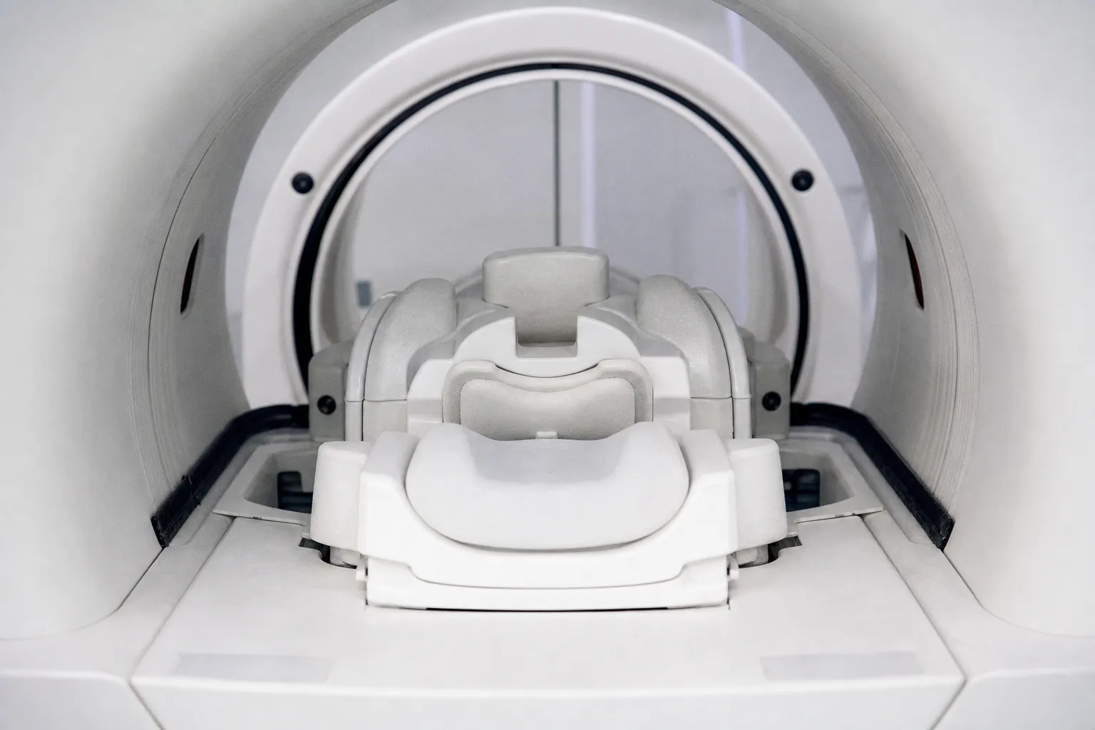
A change in head orientation alters the relationship between tissue susceptibility, RF transmit fields, receive sensitivity, and the prescribed gradient axes. The result is not merely a blurred image. It is corrupted k-space, altered spin history, and quantitative instability.
Retrospective registration acts after that corruption has already occurred. Prospective motion correction acts during sequence execution. It measures the head position, updates slice orientation and gradient coordinates, and adjusts RF phase and frequency in real time. That distinction is the technical basis for the current interest in 7T MRI prospective motion correction methods.
The term “new standard” requires discipline. Prospective correction does not eliminate every artifact, does not fully solve non-rigid physiological motion, and does not remove the need for retrospective processing. But at ultra-high field, where spatial resolution and susceptibility effects expose every failure in the acquisition chain, real-time correction is becoming difficult to treat as an optional refinement.
The physics of real-time adaptation: beyond post-processing
A conventional retrospective motion-correction pipeline assumes that each acquired volume can be represented as a rigidly displaced version of the intended anatomy. The reconstructed images are aligned after acquisition. This works when motion is limited, the contrast is stable, and the acquisition is divided into units that remain internally coherent.
Those assumptions fail in several important 7T protocols.
A 3D acquisition samples k-space over time. If the subject moves between successive portions of the trajectory, the data no longer correspond to a single rigid object in a single coordinate frame. The reconstruction combines signals acquired from different orientations. Registration can align the resulting volume with another image. It cannot reconstruct the missing consistency between individual k-space segments.
The second failure is spin history. Motion changes the spatial relationship between the tissue and the applied RF and gradient fields. Longitudinal magnetization is then prepared under one geometry and sampled under another. The artifact is encoded into the signal history before the image exists. No rigid transform can reverse that sequence of excitations.
At 7T, the problem is amplified by several coupled effects:
- Higher field strength increases susceptibility-related signal variation and local off-resonance.
- High-resolution protocols use smaller voxels, reducing tolerance to displacement.
- RF transmit inhomogeneity makes the effective flip angle spatially variable.
- Gradient-intensive sequences are more sensitive to coordinate errors and timing constraints.
- Long 3D readouts expose the acquisition to more opportunities for motion-induced inconsistency.
- Quantitative maps are sensitive not only to spatial sharpness but also to the reproducibility of signal evolution across acquisitions.
Prospective motion correction, or PMC, changes the sequence coordinates while the scan is running. The system estimates six rigid-body degrees of freedom: three translations and three rotations. It then updates the prescribed slice orientation, RF pulse phase and frequency, and gradient fields. The scanner continues to acquire data in a coordinate frame that follows the subject’s head rather than assuming that the head remains fixed inside the bore.
That is the essential mechanism. The correction is not an image-processing trick. It is an intervention at the acquisition layer.
Retrospective registration repairs image position. Prospective correction attempts to preserve signal formation itself.
This distinction also explains why prospective and retrospective methods are not interchangeable. A retrospective method can remain useful after PMC. It can correct residual volume-to-volume displacement, harmonize outputs, and support downstream analysis. But it cannot repair intra-volume blur or spin-history artifacts that were generated before reconstruction.
Tracking precision: optical systems and six degrees of freedom
The quality of a prospective correction system is bounded by its tracking loop. Measurement latency, spatial precision, rotational precision, model stability, and integration with the pulse sequence all matter. A system that detects motion accurately but updates the sequence slowly can still leave the acquisition exposed to substantial error.
In-bore optical tracking systems model the head as a rigid body. The position estimate contains six parameters:
1. Translation along the left-right axis.
2. Translation along the anterior-posterior axis.
3. Translation along the superior-inferior axis.
4. Rotation around the left-right axis.
5. Rotation around the anterior-posterior axis.
6. Rotation around the superior-inferior axis.
Reported tracking precision reaches approximately 0.1 mm for translation and 0.15 degrees for rotation. Those figures are not cosmetic specifications. At submillimeter resolution, they define whether the correction loop is operating below or above the scale of the voxel and the relevant anatomical edge.
A head-mounted marker or optical target is observed by a camera positioned inside the scanner bore. The system estimates the rigid transformation between the current and reference positions. That transformation must then be converted into scanner-compatible updates. The chain contains several possible error sources:
- Camera calibration error.
- Marker localization noise.
- Latency between measurement and sequence update.
- Coordinate-frame mismatch between the tracking system and scanner gradients.
- Mechanical vibration or marker movement relative to the head.
- Incomplete compensation for table, coil, or patient-support motion.
The scanner does not need an abstract statement that the head moved. It needs a geometrically valid correction expressed in the coordinate system of the pulse sequence. A translation affects the spatial position of the excited slab. A rotation changes the orientation of the imaging plane. The same motion can also alter the local B0 distribution, particularly at 7T, where susceptibility-induced field gradients are strong around the frontal sinuses, temporal bones, and air-tissue interfaces.
This is why optical tracking is more than a camera mounted near the patient. It is an interface between a measurement model and a real-time sequence controller.
The practical performance of optical tracking MRI motion correction depends on the temporal behavior of the full loop. The system must detect the change, estimate the transformation, communicate it, and apply the update without violating RF timing, gradient limits, or sequence reconstruction assumptions. A nominally precise tracker can still yield degraded images if its correction latency is poorly matched to the sequence.
Optical tracking versus sequence-integrated navigators
Optical systems provide an external geometric measurement. Navigators derive motion information from the MR signal itself. Each approach has a different failure profile.
| Parameter | External optical tracking | Sequence-integrated navigator |
|---|---|---|
| Primary measurement | Rigid-body position from an in-bore camera and marker | Motion or phase information derived from MR signal |
| Geometric coverage | Direct six-degree-of-freedom head tracking | Dependent on navigator design and sequence placement |
| Temporal burden | Requires camera hardware and calibration | Consumes sequence time, signal, or readout capacity |
| Sensitivity to optical obstruction | Can degrade if the marker is occluded | Not dependent on line of sight |
| B0 information | Does not directly measure field fluctuation | Can provide signal-based information about field changes |
| Integration constraint | Requires scanner and sequence interface | Must be embedded into the pulse sequence |
| Typical role | Rigid motion estimation | Motion, phase, or field-drift estimation |
Neither method is universally superior. Optical tracking provides a clean rigid-body estimate, but it does not directly measure every physiological field perturbation. An MR navigator is acquired within the imaging system and can respond to signal changes that an external camera cannot observe. It also introduces an acquisition burden and must be designed not to compromise the diagnostic sequence.
The correct comparison is not optical tracking versus navigators as competing consumer features. It is external geometry versus signal-derived state estimation. At 7T, the strongest systems increasingly combine both.
Navigating the sequence: orbital echoes and FID integration
Orbital navigator echoes, or ONAVs, embed motion estimation into the fMRI pulse sequence. They can measure and prospectively update spatial orientation across six degrees of freedom in as little as 160 milliseconds. That update interval matters because it places the correction inside the timescale of many rapid acquisitions rather than treating motion as a slow event between volumes.
An ONAV-based system typically uses a dedicated signal response to estimate the current head pose. The pulse sequence then updates the spatial orientation of subsequent excitations and readouts. The critical point is that the correction is applied before the next portion of data is acquired. The system is not asking reconstruction to reinterpret already corrupted samples.
The same logic applies to high-resolution structural imaging, though the implementation can differ. A 3D MPRAGE acquisition, a turbo spin-echo protocol, and an fMRI sequence expose motion in different ways. Their echo trains, preparation modules, phase-encoding strategies, and temporal footprints are not interchangeable. A correction method that performs well in one sequence may show different behavior in another because the motion interacts with the sequence timing differently.
FID navigators add a separate layer. A free induction decay signal can provide information about B0-field fluctuations associated with respiration and other physiological changes. At 7T, this is consequential. Rigid head motion and respiration-related field variation can coexist. Correcting only the rigid transformation leaves a residual frequency problem. Correcting only the frequency drift leaves geometric misregistration unresolved.
The combined approach uses camera-based optical PMC for rigid head motion and FID navigator correction for dynamic B0 variation. In quantitative multi-parameter mapping at 500 μm spatial resolution, this combination improved scan-rescan reproducibility in elderly subjects and patients with dementia. The significance is methodological. Reproducibility is not an aesthetic property of the image. It determines whether a measured relaxation parameter can be compared across time, subjects, and clinical groups.
A quantitative map can look sharp and still be unreliable. A small motion event can alter the signal evolution differently across acquisitions. The resulting parameter change may be interpreted as tissue biology when it is actually a sequence-state error. Prospective correction reduces that ambiguity at its source.
At 500 μm, the scanner is measuring tissue and motion at nearly the same scale. The correction loop decides which one dominates.
The integration problem is severe. Real-time corrections must coexist with gradient slew-rate constraints, RF amplifier limits, SAR restrictions, sequence timing, and reconstruction metadata. An update is only valid if the scanner can execute it without creating a new timing or encoding error.
This constrains the architecture. Prospective correction cannot be bolted onto a sequence as an afterthought. It must be represented in the pulse-programming logic, coordinate transforms, reconstruction assumptions, and safety validation. A vendor-neutral tracking device may have excellent measurement performance and still require substantial sequence-specific engineering before it produces reliable clinical data.
Quantifying clinical gains: T1, T2, and edge strength
The measurable gains reported for PMC at 7T are not uniform across contrasts. That is expected. Motion sensitivity depends on the acquisition trajectory, tissue contrast, echo structure, and spatial resolution.
In a study of non-intentional movement during 7T MRI acquisitions across 21 subjects, prospective motion correction produced a statistically significant 5.5% improvement in overall subjective image quality. The contrast-specific improvements were larger:
- High-resolution T1 imaging: 9.62%.
- T2 two-dimensional turbo spin echo: 9.85%.
- Proton-density two-dimensional turbo spin echo: 9.26%.
Objective evaluation showed a statistically significant 6% improvement in average edge strength for compliant subjects with PMC active. Edge strength is a useful complement to subjective scoring. It examines the spatial transition behavior of anatomical boundaries rather than relying solely on visual judgment. It does not represent every dimension of image quality, but it provides a more constrained measure of whether motion has softened structural detail.
These numbers should be interpreted narrowly. They support a measurable benefit under the studied acquisition conditions. They do not establish a universal percentage improvement for every 7T protocol, every subject population, or every motion pattern.
The improvement is also not equivalent to a change in signal-to-noise ratio. PMC can preserve edge localization and reduce geometric inconsistency without increasing the underlying thermal SNR. In some cases, the apparent gain comes from preventing motion-related signal mixing, not from generating more signal. The distinction matters when comparing systems or evaluating acquisition efficiency.
A useful technical separation is:
- SNR: the strength of measured signal relative to noise.
- CNR: the separation between tissue classes or pathological and normal structures.
- Edge strength: the sharpness of spatial transitions.
- Geometric fidelity: the consistency of anatomy with the intended coordinate frame.
- Quantitative reproducibility: the stability of measured parameter values across repeated acquisitions.
Prospective correction primarily targets geometric fidelity and motion-induced degradation. It can improve edge strength and perceived contrast. It may improve quantitative reproducibility. It does not make the magnet stronger, the coil more sensitive, or the sequence intrinsically more efficient.
The 7T context is important. A 5.5% overall subjective improvement can be clinically meaningful when the baseline protocol is already operating near the limit of its spatial-resolution and artifact tolerance. It can also be irrelevant if a sequence is dominated by another failure mode, such as severe susceptibility dropout, inadequate B0 shimming, RF transmit nonuniformity, or poor coil positioning.
The acquisition chain remains coupled. Motion correction cannot compensate for an unstable RF field. A high-channel-count coil cannot recover k-space consistency destroyed by motion. A better reconstruction cannot infer information that was never acquired coherently.
Hybrid strategies: prospective correction with dynamic shimming
Rigid-body tracking is necessary but incomplete. At ultra-high field, head motion can change the local B0 environment. The subject’s anatomy moves relative to the static field, and susceptibility boundaries change their spatial relationship with the magnet. The resulting field variation can degrade phase-sensitive acquisitions, alter frequency encoding, and destabilize quantitative measurements.
Dynamic shim updating addresses part of this problem. The shim system modifies compensation fields to reduce spatial variations in B0 as the head position changes. In combination with prospective motion correction, it creates a more complete control loop:
- Optical or navigator-based tracking estimates rigid motion.
- The pulse sequence updates slice orientation and gradient coordinates.
- RF phase and frequency are adjusted for the new geometry.
- Dynamic shimming responds to motion-related B0 changes.
- FID navigators monitor field fluctuations associated with respiration and other physiology.
- Retrospective processing removes residual displacement and harmonizes the final data.
This is not redundant correction. Each subsystem observes a different state variable.
A camera measures geometry. An FID navigator measures a signal response related to field behavior. Dynamic shimming changes the magnetic field environment. Retrospective registration operates on reconstructed images. Combining them can improve robustness because no single method is asked to solve every error source.
The architecture also exposes practical limits. Dynamic shimming requires compatible hardware, validated field models, and sequence support. The correction must remain within the available shim degrees of freedom. Rapid updates may be constrained by hardware response and sequence timing. At 7T, local field behavior is complex and may not be represented perfectly by a simple global correction.
Non-rigid motion remains a separate problem. Swallowing, jaw movement, respiration-related deformation, and changes in tissue configuration cannot be represented by six rigid-body parameters. Prospective correction can tolerate some of these events indirectly, but it does not convert a moving, deforming head into a rigid object.
Large or abrupt head movements also exceed the ideal operating envelope. The system may lose marker visibility, produce a poor transformation estimate, or encounter a transient field change that is not corrected by the available model. The honest claim is not that PMC removes motion artifacts. It reduces a defined class of artifacts by intervening before they are encoded into the acquisition.
What changes for protocol design
The arrival of prospective correction changes how 7T protocols should be evaluated. A sequence should no longer be judged only by nominal resolution, scan time, SAR, and contrast. Its interaction with the correction loop becomes part of the acquisition specification.
For developers and acquisition physicists, the relevant questions are concrete:
- What is the tracking latency relative to the readout and repetition structure?
- Which sequence coordinates are updated: slice position, orientation, RF frequency, RF phase, gradients, or all of them?
- Does the reconstruction retain accurate motion metadata?
- How does the method behave during intra-volume motion?
- Does the sequence contain navigators, and what acquisition burden do they impose?
- Can the system respond to B0 changes, or only rigid displacement?
- What happens when optical tracking is interrupted?
- Are corrections bounded to protect gradient, RF, and SAR constraints?
- Does the protocol preserve quantitative calibration across repeated scans?
- Which residual artifacts remain after prospective and retrospective correction are combined?
The answer cannot be reduced to a vendor checkbox. The same hardware can yield different results under different pulse sequences. A 3D isotropic anatomical protocol, a long echo-train T2 acquisition, and a rapid fMRI run present different temporal and encoding demands.
For clinical research, the endpoint should also move beyond representative images. A convincing evaluation needs objective measures, repeated acquisitions, motion-stratified analysis, and protocol-specific reporting. Average image quality can conceal a subgroup failure. A system may perform well during small compliant movements and fail during larger non-intentional displacement. Quantitative mapping should be assessed for scan-rescan stability, not just visual sharpness.
For software developers, the raw pose trace is valuable data. It can expose when the correction loop was active, when tracking confidence dropped, and how much of the scan was acquired under unstable conditions. That metadata should be preserved rather than discarded after reconstruction. It can support quality control, automated exclusion, and more honest interpretation of downstream neuroimaging results.
The new standard is an engineering threshold
Prospective motion correction is not a replacement for subject preparation, immobilization, careful sequence design, or retrospective correction. It is a way to prevent motion from becoming irreversible acquisition error.
At 7T, that distinction is decisive. High field strength increases signal potential, but it also tightens the tolerances of the system. Submillimeter imaging, long 3D trajectories, susceptibility-driven B0 variation, and quantitative mapping expose failures that lower-field protocols may hide. The scanner is not simply collecting pictures. It is executing a time-dependent mathematical model of tissue position, magnetization, gradients, RF excitation, and signal reception.
Prospective correction keeps that model closer to reality.
The evidence supports measurable gains: 5.5% overall subjective image-quality improvement, approximately 9–10% improvements in selected T1, T2, and proton-density contrasts, and a 6% improvement in average edge strength under evaluated conditions. Optical tracking can reach 0.1 mm translational and 0.15-degree rotational precision. Orbital navigators can update orientation in as little as 160 milliseconds. Combined optical and FID correction can improve reproducibility in 500 μm quantitative mapping.
Those are engineering results, not marketing language.
The remaining limitations are equally clear. Non-rigid motion persists. Dynamic field behavior is not fully captured by rigid tracking. Hardware and sequence integration remain platform-dependent. Implementation costs and broad clinical adoption are not established by the available evidence.
Prospective motion correction is therefore best understood as a new acquisition threshold, not a finished universal standard. At 7T, a scanner that ignores motion until reconstruction is already accepting avoidable corruption. The hardware may be powerful. The magnet may be stable. The coil may be excellent. If the coordinate system drifts while k-space is being filled, the data are compromised before the algorithm receives them.