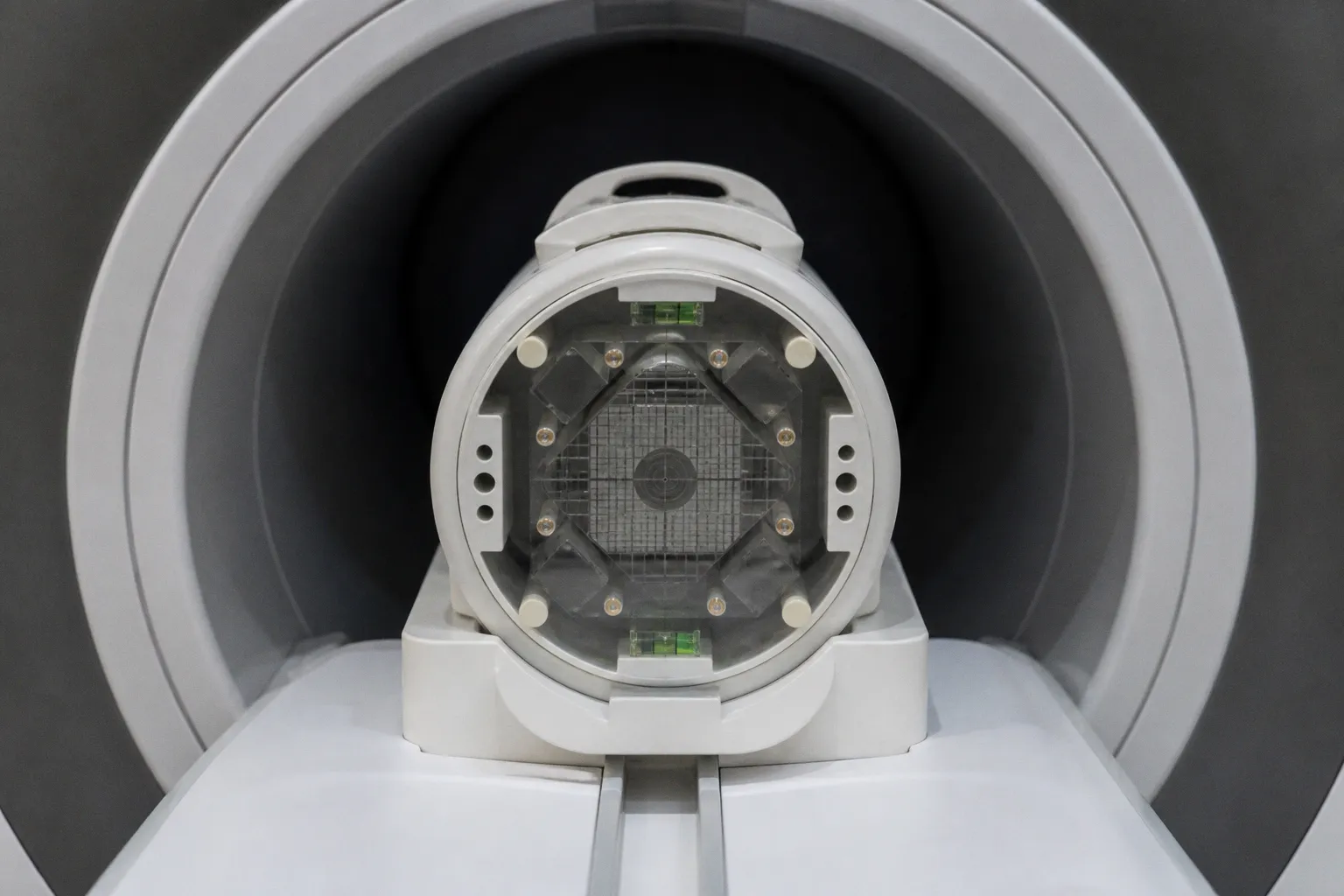
In a multi-center MRI trial, the apparent decline may come from a replaced head coil, a reconstruction software update, a sequence parameter adjustment that was never recorded, or gradual hardware degradation rather than from disease progression or treatment failure.
This is the central difficulty of managing longitudinal MRI biomarker drift in multi-center trials: the measurement is expected to follow a patient’s biological trajectory, but the instrument, protocol, and reconstruction pipeline also have trajectories of their own. Without a calibration strategy that accounts for both, a subtle change in grey-matter volume, susceptibility, perfusion, or lesion burden can become difficult to interpret—and a potentially meaningful clinical signal can be lost inside technical variance.
The physics of longitudinal drift: what changes when the patient does not
MRI biomarkers are often treated as if they were direct biological readings. They are not. They are measurements produced by an interaction between tissue properties, magnetic fields, radiofrequency transmission and reception, gradient performance, pulse-sequence design, reconstruction software, and the statistical model used to convert images into a quantitative endpoint.
That distinction matters most in longitudinal imaging studies. A cross-sectional comparison may tolerate a certain amount of site variation because each participant is analyzed within a single time point. A longitudinal endpoint is less forgiving. The question is not simply whether two scans look similar across centers; it is whether a change between two scans of the same participant reflects biology rather than a change in the measurement system.
Hardware degradation and RF coil variation
Radiofrequency coils are among the most consequential physical contributors to longitudinal MRI drift. Their sensitivity profile affects signal reception, spatial uniformity, and the relationship between tissue contrast and measured intensity. A coil replacement may be clinically routine and entirely appropriate from an engineering perspective, yet still alter the quantitative behavior of an imaging protocol.
The problem is not limited to a catastrophic hardware failure. Gradual degradation, differences between nominally similar coils, and changes in system performance after maintenance can all influence the stability of an endpoint. The effect may be especially visible in quantitative MRI, where small shifts in signal intensity or phase are translated into estimates of tissue composition, magnetic susceptibility, perfusion, or microstructural properties.
Quantitative susceptibility mapping illustrates the issue particularly clearly. QSM depends on phase information and on a chain of processing steps that includes phase unwrapping, background-field removal, dipole inversion, and reconstruction choices. A sequence parameter change, a new reconstruction release, or a head-coil replacement can therefore introduce a shift that is not obvious from a conventional visual inspection of the resulting images.
The same reasoning applies to perfusion-weighted imaging and other techniques in which timing, signal-to-noise characteristics, contrast-agent delivery, or preprocessing decisions influence the derived metric. A biomarker can be mathematically precise and still be poorly comparable across time if the acquisition conditions are allowed to drift.
A longitudinal MRI biomarker is only as stable as the measurement chain that produces it.
Software updates are part of the imaging protocol
Scanner software is sometimes treated as an operational detail rather than a component of the experiment. In a biomarker trial, that separation is unsafe. A reconstruction update may change intensity scaling, distortion correction, denoising, geometric handling, or the output format used by downstream analysis. Even if the pulse sequence appears unchanged, the image entering the biomarker pipeline may no longer be equivalent to the image acquired at baseline.
Unrecorded sequence modifications create a similar problem. Small adjustments to echo time, repetition time, acceleration, spatial resolution, bandwidth, or other acquisition parameters may be introduced to accommodate local workflow or scanner performance. In routine clinical practice, such changes can be reasonable. In a multi-center endpoint, they are protocol deviations with the potential to alter the statistical distribution of the biomarker.
This shift allows us to define drift more precisely. Drift is not merely poor image quality, and it is not synonymous with scanner failure. It is a time-dependent change in the measured endpoint that is attributable, in whole or in part, to the imaging system or analysis pipeline rather than to the participant’s biology.
That definition is practical because it points toward the right controls: document changes, measure their effect, and model the residual variation rather than assuming it is negligible.
Quantifying variance: what the Neuro/PsyGRID experience shows
The need for calibration becomes easier to appreciate when variance is separated into its components. In a multi-center calibration experiment associated with Neuro/PsyGRID, subject differences accounted for approximately 70%–80% of grey-matter variance. At the same time, center, subject, and error variance together represented more than 90% of the total variance.
The important point is not that the subject signal is weak. Individual biological differences clearly contribute a large share of the observed variation. The point is that center effects and measurement error remain substantial enough to influence statistical power and interpretation, particularly when the expected treatment effect is modest or when the endpoint is intended to detect gradual change.
In a trial, those sources of variance can interact. If one site contributes scans with a slightly different intensity distribution and another site changes its reconstruction software halfway through recruitment, the resulting pattern may resemble a treatment-by-time interaction. If treatment arms are not evenly distributed across centers, the problem becomes more serious: technical variation can become partially confounded with the clinical comparison.
Why cross-sectional normalization is not enough
A reference standard derived from a single time point can help characterize differences between scanners, but it cannot by itself guarantee that patient-level change is stable over time. Longitudinal endpoints require repeated evidence that the scanner and pipeline remain comparable across the entire study period.
This is where phantom-based MRI normalization becomes valuable. A phantom provides a controlled object with known or monitorable properties, allowing investigators to distinguish a change in the imaging system from a change in human tissue. It does not reproduce every feature of a living brain, and it cannot replace participant-level quality control, but it provides an anchor for detecting technical movement before that movement is mistaken for biology.
For QSM, the challenge is particularly important because susceptibility estimates are sensitive to acquisition and reconstruction decisions. A site modification that is not captured in the trial record may not produce an obvious failure flag, yet it can still shift the quantitative endpoint. The calibration plan therefore needs to record not only whether an image was acquired, but how it was acquired and processed.
Variance should be modeled, not simply discarded
Excluding an entire site after a late-stage quality review may appear conservative, but it can also reduce statistical power and introduce its own bias. A more mature approach combines prevention with modeling.
Voxel-level statistical models can help estimate the contribution of site, subject, time point, and residual error to the observed signal. Depending on the endpoint and trial design, investigators may use harmonization methods, mixed-effects models, scanner covariates, batch indicators, or site-specific calibration terms. The correct choice depends on the biological question and on whether the technical variation is separable from the treatment effect.
The model should never become a substitute for acquisition discipline. Statistical harmonization cannot reliably reconstruct information that was never recorded, and it cannot guarantee that software normalization has removed a physical change in the scanner. It is most useful when paired with a well-documented protocol and independent evidence from phantoms and quality-control scans.
A systemic calibration protocol for multi-center studies
A robust calibration plan begins before the first participant is scanned. The most useful protocols are not necessarily the most elaborate; they are the ones that make deviations visible, assign responsibility clearly, and create a record that can be interpreted months or years later.
A practical framework usually includes the following elements:
1. Write an imaging manual that describes the endpoint, not only the sequence.
The manual should specify acquisition parameters, positioning, coil configuration, reconstruction requirements, acceptable deviations, export formats, anonymization procedures, and the processing pathway used to derive the biomarker. For quantitative endpoints, it should also define which parameters are fixed and which may be adjusted only through documented approval.
2. Run dummy scans before recruitment begins.
Dummy runs expose differences in operator workflow, participant positioning, scan timing, data transfer, and preprocessing. They are especially valuable when several vendors, scanner generations, or local reconstruction environments are involved. The purpose is not merely to confirm that a sequence can run; it is to confirm that the entire chain produces analyzable and comparable data.
3. Acquire phantom scans at a defined cadence.
Phantom measurements create a time series for the scanner itself. The study team can monitor changes in signal stability, geometric fidelity, susceptibility-related measures, and other properties relevant to the endpoint. A single baseline phantom scan is useful, but repeated scans are what reveal drift.
4. Record every technical intervention.
Coil replacements, service visits, software upgrades, gradient calibration, sequence edits, reconstruction changes, and unusual scanner behavior belong in the trial record. The date and nature of the intervention should be linked to the imaging data so that a sudden change in the biomarker distribution can be investigated rather than treated as unexplained noise.
5. Monitor quality during recruitment rather than after database lock.
Ongoing quality control can identify a site-specific shift while corrective action is still possible. Monitoring should include image-level review, quantitative summaries, phantom trends where available, and checks for missing or inconsistent metadata.
6. Standardize data transfer and file handling.
A biomarker can be compromised by a missing series, altered scaling, incorrect orientation, incomplete metadata, or an export process that differs between sites. Data transfer procedures should therefore be tested during the dummy phase and audited during the study.
7. Define escalation rules before a problem occurs.
The team should know when a deviation requires a repeat scan, technical review, site retraining, a new calibration run, or a statistical adjustment. Decisions made under pressure after a drift signal has emerged are more likely to be inconsistent.
A useful imaging manual does not pretend that all scanners are identical. It defines the level of equivalence required for the clinical endpoint and makes the remaining differences measurable.
| Calibration element | What it controls | What it cannot replace |
|---|---|---|
| Imaging manual | Acquisition parameters, positioning, reconstruction and transfer procedures | Physical performance checks |
| Dummy run | Operator workflow, end-to-end data handling and protocol feasibility | Longitudinal monitoring during recruitment |
| Phantom scans | Scanner stability and technical trend detection | Biological interpretation of participant images |
| Change log | Traceability after service, coil or software interventions | Direct measurement of the intervention’s effect |
| Voxel-level modeling | Site, subject, time and residual variance | Prevention of undocumented protocol changes |
| Ongoing QC | Early detection of image and biomarker abnormalities | A complete validation study for a new endpoint |
Correcting spatial and gradient non-linearity
Spatial accuracy becomes increasingly important as imaging moves toward higher resolution and as biomarkers depend on precise regional measurements. Gradient non-linearity can produce geometric distortions and spatial misregistration, which may influence cortical thickness, lesion volume, tract-based measures, and voxel-wise comparisons between time points.
In a high-resolution gradient system, calibration reduced gradient scaling errors by an order of magnitude and corrected displacements greater than 100 micrometres associated with gradient non-linearity. That scale of correction is not an abstract engineering achievement. In a longitudinal study, a systematic spatial displacement can change which anatomical tissue is sampled, alter the boundaries of a segmented structure, or create an apparent regional change when the underlying tissue has remained stable.
Consider the implications for a trial endpoint based on small focal lesions or subtle cortical degradation. If the same anatomical location is not represented consistently across visits, the analysis may attribute a geometric difference to disease biology. Registration can reduce this problem, but registration is not a universal remedy. It operates on images that may already contain distortion, intensity changes, or contrast differences.
Gradient calibration should therefore be treated as part of endpoint validation. The relevant question is not only whether the scanner produces images that appear acceptable to a radiologist, but whether its spatial behavior is sufficiently stable for the measurement being used.
This matters across organ systems. In cardiac MRI, a small geometric or timing inconsistency may affect wall-thickness estimates, chamber volumes, or regional motion analysis. In oncology MRI, distortion and protocol variation can influence lesion dimensions and treatment-response assessment. In brain imaging, the same issues affect regional morphometry and voxel-wise longitudinal comparisons.
Operational safeguards: the period after a scanner upgrade
A scanner upgrade is often the moment when a study’s calibration discipline is tested. The upgrade may improve image quality, shorten acquisition time, or correct an engineering limitation. None of those benefits guarantees continuity with the pre-upgrade data.
The correct response is not to assume that the new system is either equivalent or unusable. It is to characterize the transition. Before returning to participant scanning, the site should repeat the relevant phantom acquisitions, perform a technical comparison against the prior configuration where possible, and rerun the dummy workflow. If a new reconstruction version is introduced, the study team should establish whether historical raw or reconstructed data can be processed consistently, or whether a bridging strategy is required.
The same principle applies after replacing an RF head coil. A replacement can restore expected performance while still changing the sensitivity profile. The event should be logged, followed by quality-control scans and an assessment of whether the quantitative endpoint has shifted. Treating routine maintenance as biologically neutral is not adequate for a longitudinal biomarker program.
When a protocol deviation becomes an endpoint problem
Not every deviation invalidates a scan. The clinical and statistical consequences depend on its nature, duration, and relationship to the endpoint. A minor positioning difference may have little effect on one measurement and a substantial effect on another. A software update may leave a conventional anatomical sequence visually unchanged while altering a quantitative map.
The decision should be based on evidence rather than on the appearance of the images alone. A useful review asks:
- Did the deviation change the acquisition parameters or only the local workflow?
- Is the affected scan part of the primary endpoint or a supporting measure?
- Did the change occur at one site, across all sites, or only during a defined period?
- Do phantom or participant-level QC metrics show a corresponding shift?
- Can the affected data be recalibrated, reprocessed, or modeled without obscuring treatment effects?
- Is the deviation associated with treatment allocation, visit number, or recruitment stage?
This kind of review protects the study from two opposite mistakes. The first is dismissing a technical shift as harmless because the images look clinically readable. The second is discarding potentially useful data without investigating whether the deviation can be quantified and corrected.
Calibration is not a one-time certificate of scanner quality; it is a longitudinal observation of the measurement system.
From harmonization to clinically credible biomarkers
Quantitative MRI harmonization is often described as a computational problem, but its clinical meaning is broader. A harmonized endpoint should preserve biological differences between participants while reducing variation that arises from the center, scanner, acquisition protocol, or processing pipeline. If the correction removes both technical and biological signal, the resulting biomarker may look stable while becoming less informative.
That balance is especially delicate when the study seeks to detect slow progression. Subtle degradation may unfold over years, while scanner changes can occur between two visits. Cognitive reserve, disease stage, medication exposure, and comorbidity can all influence the biological trajectory, but none of these factors can be interpreted confidently if the measurement baseline is moving.
A mature clinical research workflow therefore connects three layers:
- Physical calibration, including scanner performance, RF coil behavior, gradient accuracy, and phantom stability.
- Protocol governance, including the imaging manual, dummy runs, deviation logs, and standardized data transfer.
- Statistical interpretation, including variance decomposition, site-aware modeling, and prespecified handling of technical transitions.
Each layer answers a different question. Physical calibration asks whether the system is behaving consistently. Protocol governance asks whether the study is being conducted consistently. Statistical modeling asks how much of the remaining variation should be attributed to site, participant, time, or error.
No single layer can carry the entire burden. Software harmonization alone cannot eliminate longitudinal MRI biomarker drift when physical calibration is absent. A phantom cannot tell investigators whether a participant’s cognitive decline is real. A sophisticated mixed-effects model cannot recover the meaning of an undocumented sequence change.
Building the calibration record
For a clinical trial or longitudinal imaging cohort, the calibration record should be treated as part of the scientific dataset rather than as administrative background. It should allow an analyst to reconstruct the technical history of every relevant scan:
- scanner manufacturer, model and hardware configuration;
- RF coil identity and replacement dates;
- software and reconstruction versions;
- sequence parameters and approved deviations;
- phantom acquisition dates and results;
- gradient or geometric calibration findings;
- dummy-run outcomes;
- quality-control decisions and repeat scans;
- data-transfer and preprocessing versions.
This record supports reproducibility, but it also improves clinical judgment. When a biomarker appears to change unexpectedly, the team can compare the biological trajectory with the technical timeline. The ability to say that a shift began after a defined hardware or software event is far more useful than a general statement that the site exhibited higher variance.
The practical endpoint: confidence in change over time
The value of an MRI biomarker is not simply that it can be measured. It is that a change in the measurement can be interpreted with reasonable confidence. In multi-center trials, that confidence depends on whether the study can distinguish biological progression from the accumulated effects of hardware, software, protocol, and site behavior.
The Neuro/PsyGRID calibration experience illustrates why this distinction matters: even when subject differences explain the largest share of grey-matter variance, center and error components remain large enough to shape the endpoint. High-resolution systems show that gradient non-linearity can produce spatial errors beyond 100 micrometres before calibration. QSM demonstrates how unrecorded sequence, reconstruction, and coil changes can compromise quantitative integrity. These are not isolated technical curiosities; they are part of the causal pathway between a patient’s tissue and the number reported in a trial database.
The most defensible approach is therefore continuous and layered: define the protocol, perform dummy runs, use phantom scans, monitor quality, document interventions, calibrate spatial behavior, and model the variance that remains. This work may not make the imaging system perfectly static—and no serious biomarker program should promise that it will—but it makes change more interpretable.
That is the point at which MRI software and clinical research genuinely meet. The goal is not to create a number untouched by reality. It is to create a measurement whose relationship with reality remains visible across sites, scanners, upgrades, and years of patient follow-up.