The sequence gets adjusted because somebody needs to fit the protocol into a tighter slot. Reconstruction software receives an update. A site replaces a head coil and calls it routine maintenance.
The spreadsheet, naturally, records none of this with the urgency it deserves.
Quantitative susceptibility mapping is attractive because it turns phase information into a quantitative estimate associated with tissue iron, myelin, and calcium. That makes QSM relevant to multiple sclerosis, neurodegeneration, vascular disease, and other longitudinal research programs. But a number is not automatically a biomarker. It becomes one only when the number remains interpretable across sites, scanners, operators, visits, and software versions.
That is the operational problem behind QSM biomarker drift in multi-center trials: distinguishing biological change from measurement-system change. The former may be the endpoint. The latter is usually just expensive noise wearing a lab coat.
Why QSM drift is a systems problem, not merely a reconstruction problem
The conventional sales pitch for quantitative MRI is straightforward: acquire the data, reconstruct the susceptibility map, measure a region of interest, and compare values over time. The workflow in an actual research network is less elegant.
A QSM pipeline depends on several linked stages:
- phase acquisition and sequence parameters;
- scanner field strength and hardware configuration;
- vendor-specific implementation details;
- phase unwrapping and background-field removal;
- dipole inversion;
- reference region and susceptibility convention;
- ROI definition and segmentation;
- software version and processing environment;
- quality control and exception handling.
Any one of these can shift the resulting value. More importantly, they can shift it differently in different brain regions. A pipeline may behave acceptably in deep gray matter and become less stable near tissue interfaces or regions affected by susceptibility artifacts. A site may produce clean-looking maps while still delivering values that are not directly exchangeable with another site.
This is where the phrase “standardized protocol” often does too much work. A shared acquisition prescription is necessary, but it is not the same as a harmonized measurement system. If one site reconstructs with MEDI+0 and another uses a vendor-integrated deep-learning method, the sequence label alone does not rescue comparability. The scanners may both be called 3T. The maps may both use the same color scale. The underlying measurement behavior can still diverge.
A QSM biomarker does not drift because the biology became inconvenient. It drifts because the measurement chain was treated as a detail.
The distinction matters most in longitudinal studies. Suppose a participant returns after twelve months and the susceptibility value changes. That change could reflect iron accumulation, demyelination, calcium-related effects, disease progression, treatment response, or ordinary variation introduced by acquisition and reconstruction. Without a controlled pipeline, the endpoint becomes a negotiation between biology and infrastructure.
Infrastructure usually has more votes.
What multi-center data actually tell us
The available multi-center evidence is both reassuring and cautionary. Reassuring, because standardized QSM can achieve very high agreement under controlled conditions. Cautionary, because the same datasets show how quickly variability expands as the measurement range and operating conditions become more demanding.
A multi-center phantom study included 12 clinical and three preclinical scanners spanning 1.5T, 3T, 7T, and 9.4T systems. Using gadolinium phantoms and the MEDI+0 reconstruction approach, the measurements showed a linear relationship with an \(r^2\) above 0.99. The reported intraclass correlation coefficient was 0.991, with a 95% confidence interval reported as 0.973 to 0.99.
That is the kind of result that makes a protocol committee briefly optimistic. It demonstrates that cross-platform QSM measurement can be tightly aligned when the input material, reconstruction method, and calibration framework are controlled.
But the phantom results also contained a less comfortable detail. Measurement standard deviation increased from 32 ppb to 230 ppb as measured susceptibility rose from 0.26 ppm to 3.56 ppm. Bland–Altman limits of agreement ranged from approximately −210 ppb to 200 ppb.
In other words, agreement is not a single property of the pipeline. It depends on where the measurement sits in the susceptibility range. A reconstruction that behaves well around a low-susceptibility target may show wider dispersion at higher values. That is not a reason to abandon QSM. It is a reason to stop treating one global reproducibility number as a universal warranty.
The difference between precision and transportability
A pipeline can be precise at one site and poorly transportable across sites.
Precision asks whether repeated measurements under similar conditions stay close together. Transportability asks whether the same biological or phantom target produces comparable values when the scanner, site, operator, and processing environment change.
These are related, but not interchangeable.
A single-center study can report excellent repeatability while offering limited evidence for a multi-center trial. Conversely, a harmonized multi-center pipeline may show a wider range of values than a tightly controlled single-site experiment while still being suitable for a clinical endpoint.
For trial design, the practical questions are more demanding than “Is QSM reproducible?”
- What is the expected error at the susceptibility range relevant to the endpoint?
- Does error differ by ROI?
- Does it differ by scanner vendor or field strength?
- Is the error stable across software releases?
- Can a site be identified as an outlier before its data reach the primary analysis?
- What magnitude of biological change must be detected above the measurement floor?
Those questions belong in the protocol, not in the post hoc discussion after the database has been locked.
Phantom calibration: the part everyone approves and nobody wants to schedule
Phantom calibration is rarely the most glamorous item in a clinical research timeline. It also tends to survive budget review only until someone notices that it requires scanner access, shipping logistics, standardized positioning, acquisition time, central review, and a response plan for failures.
That is exactly why it matters.
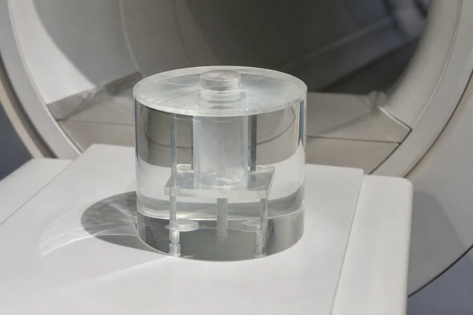
A phantom is not a decorative object placed in the scanner to make the methods section look mature. It is a reference instrument for detecting whether the measurement chain is behaving consistently. In QSM, a calibration phantom can expose discrepancies that are invisible in routine image review. Two maps can appear visually similar while their quantitative values diverge enough to complicate a longitudinal endpoint.
The strongest phantom result in the available evidence—the ICC of 0.991 across scanners from 1.5T to 9.4T—was achieved within a defined acquisition and reconstruction framework. The number is evidence for the framework, not permission to mix arbitrary pipelines and assume that physics will sort it out.
A useful calibration program should establish three layers of control:
1. Site qualification before enrollment.
Each scanner should acquire the agreed phantom and human test data before contributing participant scans. The central team can then assess whether the site falls within the expected measurement envelope.
2. Routine monitoring during the study.
Calibration performed only at study launch will not detect every later change. Hardware service, coil replacement, software updates, sequence edits, and reconstruction changes can all create a new baseline.
3. Triggered requalification.
A site should repeat calibration after defined technical events rather than waiting for unexplained endpoint behavior. The trigger can be a scanner upgrade, coil intervention, protocol modification, or a persistent QC deviation.
The point is not to build a perfect laboratory around every scanner. The point is to make technical change visible early enough that it can be handled as a documented event rather than discovered as an unexplained biomarker trend.
What to record with every QSM acquisition
A QSM dataset without acquisition and processing metadata is a future argument with missing exhibits. At minimum, the trial should retain:
- scanner manufacturer, model, field strength, and software version;
- coil configuration and relevant hardware changes;
- sequence parameters, including echo times, repetition time, flip angle, resolution, and acceleration;
- orientation and positioning information;
- phase preprocessing choices;
- phase unwrapping method;
- background-field removal method;
- dipole inversion algorithm and regularization settings;
- reference convention for susceptibility values;
- segmentation and ROI generation method;
- reconstruction software version and container or environment identifier;
- QC status, reviewer, and reason for any exclusion or correction.
This is not bureaucracy for its own sake. It is the minimum information required to determine whether a value changed because a participant changed or because a pipeline quietly changed underneath them.
Traveling brain studies expose the vendor problem
Phantoms are essential, but they do not behave like human brains. They are stable, geometrically defined, and free of motion, anatomy, vascular pulsation, and disease-related heterogeneity. Human reproducibility studies are therefore the more uncomfortable test.
In a traveling brain evaluation, six subjects were scanned on 3T systems from two vendors. Quantification errors varied by ROI, ranging from 0.001 to 0.017 ppm. That range is not a trivial footnote. It says that inter-vendor discrepancy is not one fixed offset that can be removed with a single correction factor.
The ROI matters. The anatomy matters. The susceptibility environment matters. The algorithm’s behavior at the edges of structures matters. A global harmonization coefficient may look attractive in a statistical model, but it can conceal region-specific failure.
A separate standardized QSM protocol across nine sites using 3T systems from three vendors reported ROI-dependent susceptibility variability between 0.005 and 0.025 ppm in healthy participants. Again, the headline is not that multi-center QSM is impossible. The headline is that the uncertainty has structure. It is not random confetti scattered equally over the brain.
Vendor variation is not limited to the scanner console
When teams say “vendor effect,” they often mean differences in field strength, sequence implementation, gradient performance, or reconstruction behavior. In practice, the effect can be distributed across the entire workflow.
Consider a typical research network:
- One site exports raw phase data in a familiar format.
- Another performs a vendor-side correction before export.
- A third has a local script that converts phase data with undocumented assumptions.
- Central processing receives files that share a naming convention but not necessarily a measurement history.
The API handshake succeeded. The data are still not necessarily comparable.
Software is particularly good at hiding this problem. A reconstruction update may improve visual quality, reduce streaking, or accelerate processing. Those are useful changes. They can also alter quantitative values. If the trial treats the new software release as a harmless IT patch, the study may introduce a discontinuity without recording one.
For this reason, reconstruction pipelines should be versioned like clinical-grade software, not managed like a folder of useful scripts on a graduate student’s workstation. Every release should have a defined validation set, a change log, and a rule for whether historical data will be reprocessed.
When the endpoint is smaller than the noise
The clinical argument for QSM usually involves subtle change. That is where the biomarker is potentially valuable—and where drift becomes most expensive.
In repeated brain scans of healthy participants and people with multiple sclerosis at 1.5T and 3T, mean inter-scan QSM differences were reported below 1.24 ppb in healthy volunteers and below 4.15 ppb in participants with MS. These findings support the possibility of highly repeatable measurements under controlled conditions.
They should not be interpreted as a universal error budget for every QSM trial. The reported differences come from specific study designs, scanners, regions, and processing conditions. A multi-center oncology or neurodegeneration study with broader protocol variation may experience a different uncertainty profile.
Still, the figures make the underlying point clear: when the expected biological effect is small, a few parts per billion can matter. The endpoint does not need a dramatic failure to become unreliable. It only needs technical variation to approach the effect size the study was built to detect.
This creates several consequences for trial statistics and operations.
1. Define the measurement floor before powering the study
The sample-size calculation should not rely only on the anticipated biological effect. It should incorporate repeatability, between-site variance, ROI-specific error, and any expected site or vendor effects.
If the endpoint is based on change from baseline, the covariance between visits matters. If the same participant is scanned on different hardware, that pairing may not behave like a simple repeated measure on the same scanner. The statistical model needs to reflect the acquisition reality rather than the preferred diagram in the protocol.
2. Separate QC failures from biological outliers
An extreme QSM value may indicate unusual pathology. It may also indicate phase-wrap failure, poor background-field removal, motion, segmentation error, or a reconstruction problem. Automatically treating every outlier as biology is a reliable way to promote pipeline defects into scientific findings.
Central review should inspect both the quantitative output and the intermediate quality indicators. A visually plausible map is not sufficient, but a numerical threshold without anatomical context is not sufficient either.
3. Preserve the distinction between exclusion and correction
Removing a bad scan can protect the analysis, but it can also introduce bias if failures are more common at particular sites, visits, or disease stages. Correcting a value can be even more dangerous if the correction is not prospectively defined.
A trial should specify what constitutes a failed acquisition, what can be repeated, what can be reprocessed, and what must remain flagged. Otherwise, every difficult case becomes an improvised committee decision. Committees are useful. They are less useful when they are functioning as undocumented software.
4. Treat site as an analytical variable
Site effects should not be hidden inside a generic residual term if the study is explicitly multi-center. The analysis may need scanner, vendor, field strength, acquisition batch, and processing version as covariates or hierarchical effects, depending on the endpoint and design.
The objective is not to statistically erase every difference. It is to model known sources of variation honestly and avoid claiming a biological signal that is really a site transition.
The most dangerous QSM outlier is not the absurd value. It is the plausible value produced by a changed pipeline.
Harmonizing the reconstruction pipeline without freezing progress
Standardization does not mean refusing to update software forever. It means controlling change so that improvement does not become confounding.
There are two common failure modes.
The first is excessive flexibility: each site uses the reconstruction method it prefers, central analysis receives whatever output arrives, and harmonization is attempted later with a statistical patch. This maximizes local convenience and minimizes interpretability.
The second is rigid stagnation: the trial locks an old pipeline and treats any update as forbidden, even when a security, compatibility, or reconstruction issue requires intervention. This preserves consistency by turning the study into an archaeological site.
A more practical model is a controlled pipeline with explicit release management.
Freeze the measurement definition, not necessarily every tool
The trial should define what the biomarker means operationally:
- which QSM quantity is analyzed;
- which reference convention is used;
- which anatomical regions are primary;
- how ROIs are generated and reviewed;
- which preprocessing and inversion assumptions are mandatory;
- what QC thresholds apply;
- what constitutes a valid longitudinal comparison.
Once those definitions are fixed, software changes can be evaluated against them. A new algorithm must demonstrate acceptable agreement, stability, and failure behavior before it becomes part of the production workflow.
Prefer central reconstruction when the raw data allow it
Central reconstruction reduces one major source of variation: local implementation. Sites still differ in acquisition, hardware, and raw-data export, but the processing logic is no longer reinvented at every hospital.
That does not eliminate the need for site QC. It does reduce the number of silent forks in the pipeline.
If central reconstruction is not feasible, the alternative is not to trust each site’s software output by default. It is to distribute a versioned, validated environment—ideally with locked dependencies, documented settings, test data, and an auditable processing record.
The goal is not technological purity. It is to prevent the classic workflow bottleneck in which the imaging core spends half the trial asking sites which version of a script produced a given number.
Build a bridge set for every pipeline release
Before a reconstruction release is deployed, process a representative bridge dataset containing:
- phantom scans across the relevant susceptibility range;
- repeated human scans;
- multiple vendors and field strengths if they are in scope;
- difficult anatomical regions;
- cases with known motion or artifact patterns;
- the exact ROIs used for the primary endpoint.
Compare the new and old outputs quantitatively, not just visually. A release may produce nearly identical maps while shifting regional values enough to matter. If the difference is systematic and understood, the study can decide whether to reprocess historical data, include a version effect, or maintain separate calibrated eras.
No one enjoys reprocessing. Everyone enjoys it more than explaining an unexplained step change in the primary biomarker.
A practical drift-monitoring framework
A multi-center QSM trial benefits from treating calibration as a continuous control loop rather than a one-time acceptance test. The workflow can remain operationally simple if the decisions are defined before the first participant scan.
| Monitoring layer | What it catches | Useful action |
|---|---|---|
| Phantom scan | Scanner, coil, sequence, or reconstruction shift | Compare against site baseline; trigger requalification if outside limits |
| Traveling human or repeat-subject scan | ROI-specific inter-vendor and inter-site discrepancies | Estimate transportability and regional error |
| Raw-data and metadata audit | Missing parameters, undocumented changes, inconsistent exports | Block analysis-ready status until the acquisition history is complete |
| Central image QC | Motion, phase artifacts, background-field failure, segmentation errors | Accept, repeat, reprocess, or exclude under predefined rules |
| Pipeline regression test | Software release changes and dependency drift | Approve, revise, or reject the new processing version |
| Longitudinal site dashboard | Gradual drift, visit effects, site-specific outliers | Investigate before the problem contaminates the endpoint |
The key is escalation. A dashboard that only displays red and green indicators is not quality control; it is decorative anxiety. The team needs a documented response for each class of deviation.
For example, a phantom shift may require a repeat scan. A repeat failure may require service review. A software change may require reprocessing of a defined historical batch. A segmentation problem may require manual adjudication. These are different failures and should not be compressed into a single field called “QC status.”
Use ROI-specific limits rather than one global threshold
The evidence from traveling human studies and multi-site standardized protocols points repeatedly to ROI-dependent variability. That should affect the QC design.
A single whole-brain tolerance can miss a problem concentrated in a vulnerable structure. Conversely, a threshold calibrated to a difficult ROI may generate unnecessary alarms for a stable one. Primary regions should have their own expected ranges, repeatability estimates, and review rules.
This is especially important when a study measures structures with different susceptibility behavior or different proximity to air-tissue interfaces. The map may be technically valid overall while the region used for the endpoint is not reliable enough for interpretation.
What this means for clinical translation
QSM is often described as a promising imaging biomarker because it connects MRI physics with tissue composition. That promise is real, but translation requires more than a biologically plausible signal and a statistically significant group difference.
A clinical-trial biomarker must survive operational stress:
- different scanners;
- staff turnover;
- acquisition delays;
- protocol deviations;
- software updates;
- site onboarding;
- participant motion;
- repeat visits;
- central data transfers;
- analysis changes under deadline pressure.
The more complex the trial, the less useful it is to describe the biomarker as a single algorithm. It is a distributed measurement service. The scanner, sequence, reconstruction, segmentation, QC, and analysis model all contribute to the final number.
That framing also changes how teams should allocate effort. Developers may focus on inversion quality and artifact suppression. Radiologists may focus on interpretability and reading-room burden. Trial statisticians may focus on variance components. Imaging core staff may focus on throughput and exception handling. All of these concerns are legitimate, but the biomarker fails if they remain disconnected.
A reconstruction algorithm that improves map quality but doubles processing failures is not automatically an advance. A pipeline with excellent ICC in phantoms but no mechanism for handling vendor upgrades is not trial-ready. A segmentation model with impressive validation metrics but inconsistent behavior across disease-related atrophy patterns can still undermine a longitudinal endpoint.
The useful question is therefore not whether QSM can be standardized in theory. It is whether the complete workflow can be operated, monitored, and audited for the duration of the study.
The cautious conclusion
The evidence supports a constructive position. QSM can achieve strong cross-scanner agreement and high repeatability when acquisition and reconstruction are standardized. The phantom ICC of 0.991 demonstrates what a controlled framework can accomplish. Human studies show that repeatability can also be excellent under defined conditions.
But the same evidence rejects the easy version of the story. Variability changes with susceptibility range, ROI, vendor, scanner, and processing conditions. Reported inter-site variability of 0.005–0.025 ppm and traveling-subject quantification errors of 0.001–0.017 ppm are reminders that transportability must be measured rather than assumed.
For a multi-center trial, the sensible operating model is clear:
1. qualify every site before enrollment;
2. centralize or tightly control reconstruction;
3. retain complete acquisition and processing metadata;
4. use phantoms throughout the study, not only at startup;
5. validate each software release against a bridge dataset;
6. estimate repeatability by ROI and scanner context;
7. model site and pipeline version in the analysis;
8. define failure, repeat, reprocess, and exclusion rules in advance.
That is less exciting than announcing a universal QSM standard. It is also more useful.
Biomarker drift is not an unavoidable tax on multi-center imaging. It is what happens when a quantitative measurement is deployed as if the scanner were the whole system. The scanner is only the front end. The real biomarker is the entire chain—and every link needs a version number.