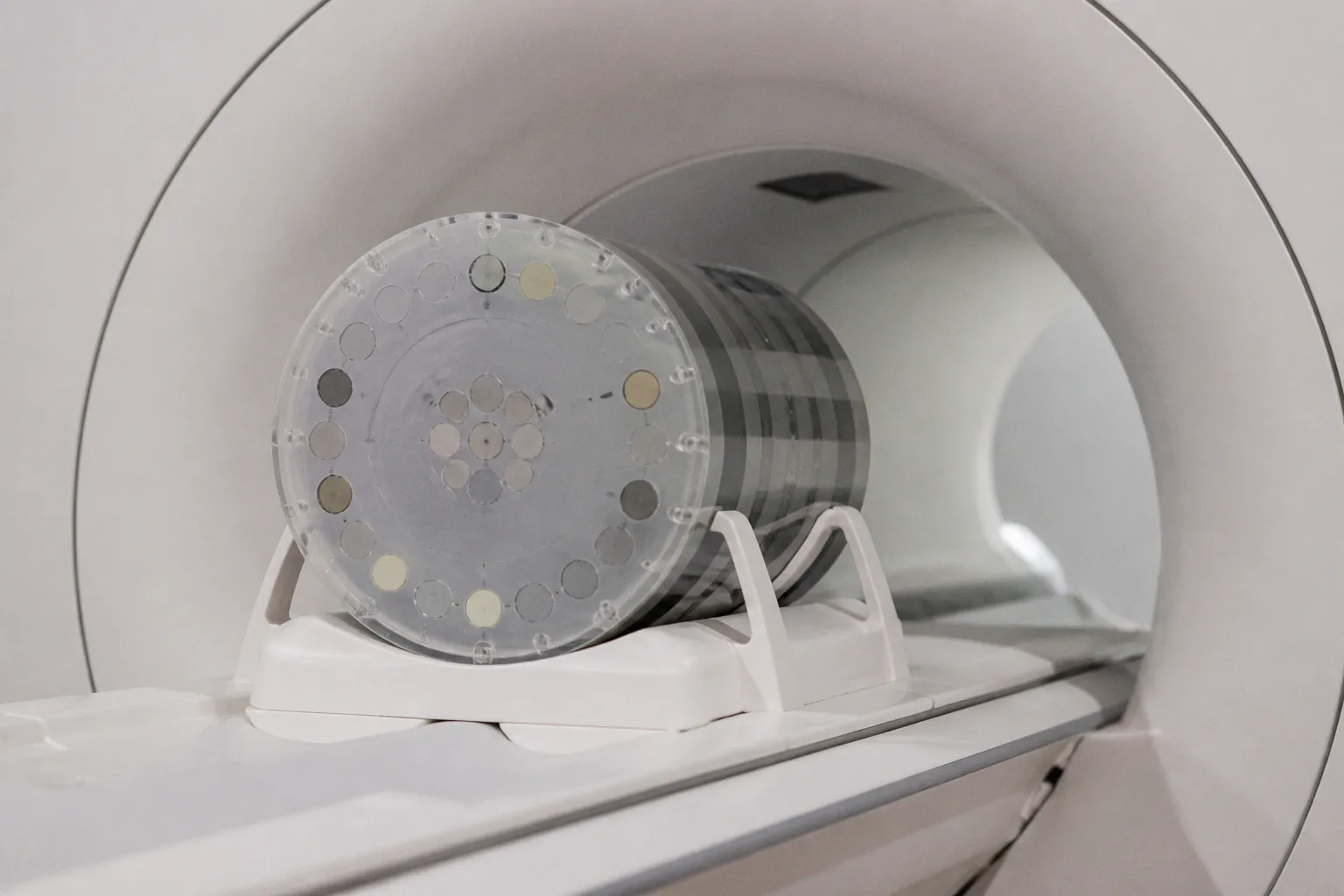
The original 3 Tesla magnet is replaced with a newer model — same vendor, same field strength, ostensibly the same protocol — and yet the hippocampal volumes that had been trending downward so gently over three years of follow-up suddenly shift, almost imperceptibly, by two to four percent. The intra-class correlation coefficient, the reassuring statistic that the protocol team points to in the steering committee meeting, still reads above 0.8. Nothing, on the surface, looks broken. Everything, beneath it, has changed. The question facing every translational neuroscience group working with quantitative MRI biomarkers today is not whether a hardware transition introduces bias, but how to check MRI harmonization after scanner upgrades with enough rigor to keep the biological signal intact.
This is not a hypothetical concern. In one widely cited comparison, upgrading from a Siemens Verio to a Skyra scanner at the same institution introduced statistically significant differences in gray matter measurements across at least 67% of regions of interest, with magnitude shifts in the 2% to 4% range — even as intra-class correlation coefficients exceeded 0.8. Consider the implications: the very statistics that suggest reliability are exactly the ones that allow systematic drift to slip past. For any trial that relies on longitudinal change as its primary endpoint, this is the place where a decade of careful phenotyping can begin to erode.
Quantifying the Hidden Impact of Hardware Transitions
Hardware transitions look, on paper, like administrative events. A service contract ends, a new console arrives, a sequence gets re-tuned, and life at the imaging core resumes. But every magnet, every gradient coil, every receiver array, and every reconstruction algorithm has a fingerprint, and that fingerprint is woven into the voxel intensity long before any radiologist looks at the image. When a scanner is swapped, the fingerprint changes — sometimes by design (a new parallel imaging factor, a refined shim routine), sometimes by accident (a different coil loading configuration, an updated software patch that quietly re-scales the dynamic range).
This matters because quantitative imaging biomarkers are precisely the kind of metrics that depend on absolute, comparable intensities. A 2% shift in cortical thickness sounds small, but across a five-year trajectory of subtle neurodegeneration it is comparable to the entire expected annual rate of atrophy in a healthy aging adult. This shift allows us to mistake a hardware event for a therapeutic response, or to declare a drug futile when the molecule was, in fact, doing exactly what the preclinical data predicted.
The first practical step in checking harmonization, then, is to refuse to assume that "same vendor, same field strength" means "same measurement." It does not. The bias lives in the gradient calibration, the B1 field profile, the diffusion encoding scheme, and the reconstruction kernel — and these are precisely the components most likely to change during a platform refresh.
Where the bias actually hides
Structural T1-weighted imaging, the workhorse of volumetric studies, has long been assumed to be relatively robust to scanner effects, and in many cross-sectional analyses this assumption holds. But the moment you ask the same participant to be scanned on two different machines — or to be scanned before and after a console upgrade on the same machine — the assumption frays. Voxel intensity distributions shift. Contrast-to-noise ratios drift. Head coil geometry changes the point spread function just enough to alter the boundary between gray matter and white matter at the segmentation step, and the downstream cortical thickness estimate carries that boundary shift into every subject's record.
Diffusion tensor imaging is even more vulnerable. Fractional anisotropy, mean diffusivity, and the full set of tensor-derived metrics carry pronounced scanner effects that are almost always present, regardless of how carefully the protocol was matched. If a study relies on white matter microstructure as a biomarker — for example, in traumatic brain injury, multiple sclerosis, or early detection of dementia — and no explicit check for scanner effects has been performed in the diffusion data, the measurement is almost certainly describing the hardware as much as the biology.
The Fallacy of High ICC in Post-Upgrade Reliability
An intra-class correlation coefficient above 0.8 tells you that the rank order of subjects is preserved between scanners. It tells you almost nothing about whether the absolute measurement has quietly drifted in the same direction for everyone.
This is the single most important conceptual point in the entire harmonization literature, and it is the one most often missed in practice. The ICC is a measure of relative agreement — it answers the question, "If I rank my participants from lowest to highest on scanner A, does that same ranking hold on scanner B?" When the answer is yes, with a coefficient above 0.8, we breathe a sigh of relief and move on.
But consider the implications of this kind of reassurance. If every participant's hippocampal volume is systematically inflated by 3% on the new scanner, the rank order is preserved beautifully. The ICC remains high. The absolute values, however, are now incompatible with the historical cohort, and the longitudinal trajectory — the actual endpoint of the trial — has been silently recalibrated. Cognitive reserve estimates that depended on a stable baseline now drift with the hardware, and the patient-level decisions built on top of those estimates drift with them.
This is why post-upgrade reliability assessment requires more than a single correlation coefficient. It requires an explicit test for systematic mean shifts: paired comparisons on a representative subset of participants scanned before and after the upgrade, Bland-Altman analyses to visualize the agreement structure, and ideally a formal test of equivalence against a pre-specified equivalence margin. Without these, the high ICC is a comforting statistic that can hide exactly the bias it was supposed to rule out.
What a credible reliability battery looks like
A rigorous post-upgrade check combines at least three complementary analyses. First, voxel-wise intensity comparisons identify whether any anatomical region is shifting more than expected under the null hypothesis of "no scanner effect." Second, region-of-interest summary features — cortical thickness, subcortical volume, fractional anisotropy within major tracts — are tested for paired differences in the same participants scanned on both platforms. Third, multivariate classification models can be trained to predict scanner identity from the imaging features alone; if a classifier achieves high accuracy, the scanner has left a detectable signature in the data, and harmonization is required before pooling.
The Adjusted Rand Index offers a particularly elegant way to quantify how well a harmonization method has restored participant-level clustering. An ARI above 0.8 after harmonization, compared to a near-zero ARI before, is strong evidence that the algorithm has removed the scanner fingerprint without obliterating the biological variability that makes the cohort worth studying in the first place.
Traveling Human Phantoms as the Gold Standard for Bias Detection
The traveling human phantom is, in many ways, the cleanest experimental design available for post-upgrade harmonization validation. A small group of volunteers — typically between five and ten — is scanned repeatedly across the scanners or scanner configurations under investigation. The same individuals, the same anatomical reality, the only thing that changes is the hardware.
This design is what allows researchers to separate biological variability from measurement bias with genuine rigor. Within-subject variation across scanners reflects the hardware contribution; between-subject variation reflects the biology; the difference between the two is the signal-to-noise ratio of the entire study. Any harmonization algorithm can be benchmarked against that ground truth, and any clinical inference drawn from the harmonized data inherits the trustworthiness — or the untrustworthiness — of that benchmark.
The protocol is unglamorous and demanding. Each volunteer must be positioned carefully, the sequences must be run in matched order, and the session must be repeated enough times to estimate within-subject variance reliably. But the payoff is substantial. A traveling phantom study gives actual measurements of the same brain on different hardware — measurements that simply do not exist any other way.
What traveling phantoms reveal
In practice, traveling phantom studies tend to expose exactly the biases that routine reliability checks miss. The 2% to 4% magnitude shifts reported in the Verio-to-Skyra transition are not detected by visual inspection of the images and are only partially detected by ICC; they are exposed by paired comparisons within the same individual across platforms. The same protocol, run on the same person, on the same week, on machines that the manufacturer describes as comparable, produces measurements that are systematically different in a majority of regions.
For diffusion metrics, the effects are larger still. Fractional anisotropy and mean diffusivity are exquisitely sensitive to gradient calibration, eddy current correction, and the specifics of the diffusion encoding scheme. Without a traveling phantom baseline, there is no honest way to know how much of a longitudinal white matter change is biology and how much is reconstruction software being interpreted as biology.
Statistical and Deep Learning Approaches to Signal Alignment
Once the bias is characterized, the question becomes how to remove it without removing the signal. The harmonization toolkit has matured substantially over the past several years, and the current options span classical location-scale adjustments, empirical Bayes methods, and increasingly sophisticated deep learning approaches.
The ComBat family
The original ComBat algorithm — and its longitudinal (longCombat) and neuroimaging-specific (neuroCombat, gamCombat) extensions — has become the de facto workhorse of statistical harmonization. These methods model the scanner effect as a location and scale shift on each feature, with empirical Bayes shrinkage to stabilize estimates in small samples. In validation studies against traveling phantom data, neuroCombat, longCombat, and gamCombat have demonstrated false positive rates below 5%, which is to say they introduce minimal spurious "disease-like" signal when applied to healthy controls scanned across platforms.
The table below summarizes the principal harmonization methods and the contexts in which they tend to perform best:
| Method | Best suited to | Key strength | Important caveat |
|---|---|---|---|
| ComBat (location-scale) | Cross-sectional structural T1, ROI summaries | Simple, well-validated, low false positive rate | Can distort signal if no scanner effect is actually present |
| longCombat | Longitudinal studies with repeated measures | Preserves within-subject trajectories | Requires consistent timing of measurements across sites |
| neuroCombat | Multi-site neuroimaging pooling | Designed for voxel-wise and ROI data | Does not generalize automatically to DTI or perfusion |
| gamCombat | Studies with covariate adjustments | Handles age, sex, diagnosis covariates | More complex to tune, requires careful specification |
| Deep learning (k-space / feature space) | Dynamic range mismatch, contrast drift | Can align intensity distributions directly in image domain | Less interpretable, harder to validate against ground truth |
When deep learning earns its complexity
The classical ComBat family assumes that the scanner effect can be captured as a location and scale shift on each feature independently. For many structural measures this is a reasonable approximation. But when the scanner effect involves a change in the dynamic range of the image — a compression or expansion of the intensity histogram that does not preserve relative ordering — purely additive and multiplicative corrections begin to fail.
This is where deep learning harmonization earns its complexity. By performing operations in k-space (the raw frequency-domain representation of the MRI signal) or in learned feature space, neural network approaches can perform nonlinear transformations that align dynamic ranges across scanner systems without corrupting the clinical disease markers that make the imaging study worth doing. The reported ARI above 0.8 for participant clustering across scanners after such methods is a strong empirical signal that the approach can preserve biological structure even when simple linear corrections cannot.
Preserving Biological Variance During Algorithmic Harmonization
The question is never whether harmonization helps. The question is whether the harmonization you applied is removing the noise or erasing the signal you spent years trying to measure.
This is the deepest methodological trap in the field. Harmonization is a form of signal processing, and like all signal processing it can be applied aggressively or conservatively. Applied conservatively, it removes the scanner fingerprint while leaving the biological variance intact. Applied aggressively — or applied when no scanner effect was actually present in the first place — it can compress real differences between participants and obscure the very disease signal the study was designed to detect.
The literature is clear on the structural T1 case: harmonization applied when no underlying scanner effect exists can obscure genuine biological differences. If the cohort happens to be scanned on a single platform, or if the traveling phantom study fails to detect a meaningful scanner effect, applying ComBat or a deep learning method anyway will not make the data "more comparable" — it will make the data less honest, and any apparent consistency across sites will have been manufactured rather than measured.
The diffusion tensor imaging case is the inverse. Fractional anisotropy and related diffusion metrics consistently contain pronounced scanner effects, and harmonization is almost always required before pooling data across platforms. Skipping this step in the diffusion domain is, if anything, the more common error, because the visual appearance of the diffusion maps looks reasonable even when the quantitative values are systematically biased.
A practical decision framework
A defensible post-upgrade harmonization workflow follows roughly these steps:
1. Establish a traveling human phantom baseline across the scanner configurations involved.
2. Quantify the magnitude of the scanner effect in each imaging modality — voxel-wise for intensity, ROI-wise for derived metrics.
3. Test whether harmonization is genuinely required for each modality separately, rather than applying it uniformly out of habit.
4. Apply the appropriate harmonization method — ComBat family for structural measures where linear shifts dominate, deep learning methods for dynamic range mismatches and contrast drift, modality-specific tools for diffusion and perfusion.
5. Validate the result against the traveling phantom ground truth, confirming that biological variance is preserved (ARI above 0.8 is a useful benchmark) and that false positive rates remain within acceptable limits (below 5% for the ComBat family is a reasonable target).
The human dimension underneath the statistics
It is easy, in a methodological discussion like this one, to forget that every voxel carries a human history. The hippocampal volume being measured is the hippocampal volume of a person — perhaps someone enrolled in a trial of a new disease-modifying therapy, someone whose trajectory of cognitive reserve is being mapped against the slow degradation of neurodegeneration, someone whose family is waiting for a signal that the intervention is working.
When a scanner upgrade quietly shifts that measurement by three percent, the consequences are not abstract. A treatment effect that was real can become invisible. A biomarker that was tracking disease progression can appear to plateau. The longitudinal trajectory that anchors the entire clinical interpretation is rewritten by a hardware event that nobody intended, and the participant who returned for their year-three scan has no way of knowing that the machine has, in a quiet and literal sense, changed the answer.
This is why checking MRI harmonization after scanner upgrades is not a bureaucratic chore but a clinical responsibility. The methodological choices — whether to apply ComBat, whether to deploy a traveling phantom, whether to trust an ICC above 0.8 or to demand a paired comparison — are, ultimately, choices about how seriously the field takes the participants who agreed to be scanned year after year so that something true could be learned.
Closing Perspective
The trajectory of neuroimaging biomarker science depends on whether the community can keep its measurements honest across hardware generations. The tools exist — traveling human phantoms, statistical harmonization methods with validated false positive rates, deep learning approaches that operate in the right domain, and a clear understanding of when not to harmonize at all. What is required is the discipline to deploy them in the right order, on the right modalities, against a ground truth that the data itself cannot provide without intentional design.
The next time a scanner console is swapped, the question worth asking is not whether the new machine is "compatible." It is whether the team has built the infrastructure to detect and correct the bias that the swap will introduce — and whether the longitudinal trajectories that follow will still describe the biology they were always meant to describe.