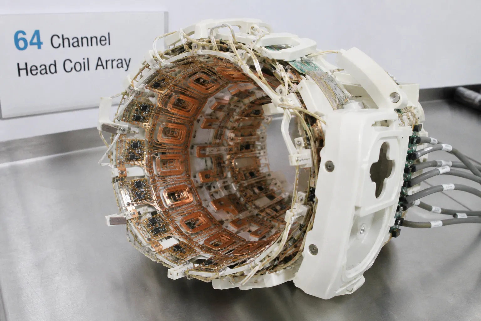
The empirical reality, however, is considerably more nuanced — and this nuance matters when a scan is being planned to detect a five-millimeter cortical lesion adjacent to eloquent cortex, or to map the hemodynamic response of the visual cortex to a flickering checkerboard. A study comparing size-matched 32- and 64-channel head coils on a 3T scanner showed a 1.3-fold increase in cortical signal-to-noise ratio with the denser array, yet essentially indistinguishable SNR in the central brain for unaccelerated imaging, a finding that has quietly shaped how academic imaging centers allocate their hardware budgets over the past decade.
The temptation is to assume that channel count scales linearly with diagnostic value. Consider the implications of what the data actually show: the geometry of the receive array, the depth of the region of interest, the parallel imaging acceleration factor, and the field strength all interact with channel count in ways that resist generalization. What follows traces those interactions, with particular attention to where the 64-channel architecture earns its premium and where the 32-channel array remains the more defensible choice.
Signal-to-noise ratio dynamics across cortical and central brain regions
The signal-to-noise ratio of a receive array is governed by two competing factors: the intrinsic noise contribution of each individual element, which tends to rise as more loops are packed into a fixed housing, and the array's ability to encode spatial information for parallel imaging, which improves with channel density. At 3T, when no parallel imaging acceleration is applied, the trade-off resolves in a way that depends almost entirely on where in the brain the measurement is being made. The cortical SNR gain of the 64-channel array — approximately 1.3-fold over a size-matched 32-channel coil — reflects the smaller, more numerous loops concentrating their sensitivity in the periphery, close to the elements themselves. Deeper structures, by contrast, see their signal averaged across many overlapping sensitivity profiles, and the gains largely cancel.
| Parameter | 32-channel array | 64-channel array |
|---|---|---|
| Cortical SNR, 3T, unaccelerated | baseline | ~1.3× higher |
| Central brain SNR, 3T, unaccelerated | baseline | comparable |
| Central brain SNR, 3T, R = 4 | baseline | ~1.2× higher |
| Cortical SNR, 3T, R = 4 | baseline | ~1.4× higher |
| 7T central brain SNR, unaccelerated | baseline | no significant gain |
| 7T cortical SNR, unaccelerated | baseline | higher |
| Achievable 2D acceleration at 7T | limited | up to 12–16-fold |
The practical consequence is that a researcher or radiologist who needs to characterize a subcortical structure — the head of the caudate, the medial temporal lobe, or the pulvinar — may not recover a meaningful SNR return from the channel-count premium. This shift allows us to redirect acquisition strategy toward parameters that do influence deep-brain fidelity: voxel size, readout bandwidth, and careful shimming. Conversely, when the clinical question is whether a small cortical lesion represents a low-grade glioma or a focal area of cortical dysplasia, the additional cortical SNR can be the difference between a confident report and a follow-up scan that delays surgical planning.
Parallel imaging performance and g-factor at high acceleration
Parallel imaging exploits the spatial sensitivity maps of the receive array to fold k-space, reducing scan time at the cost of a noise penalty described by the geometry factor, or g-factor. As acceleration factors climb, the g-factor penalty typically grows, and the noise benefit of additional channels becomes more pronounced — because the higher-dimensional encoding space provided by 64 elements is better able to disentangle the aliased signal. The same 3T comparison makes this clear: at R = 4, the 64-channel array produced approximately 1.2-fold higher SNR in the central brain and approximately 1.4-fold higher SNR in the cortex than its 32-channel counterpart. The central-brain figure is particularly informative, because it represents the unfolding of an SNR benefit that was essentially absent at R = 1.
The channel-count premium is not a property of the array in isolation — it is a property of the array in conversation with the acceleration factor.
This interaction matters most for protocols that are intrinsically acceleration-hungry. Diffusion-weighted imaging with high angular resolution, susceptibility-weighted angiography that demands very high readout bandwidth, and multi-echo MPRAGE acquisitions all benefit from the elevated R values that a 64-channel architecture can sustain without catastrophic g-factor blow-up. In clinical workflow terms, this often translates into the ability to push slice counts higher in a fixed TR, which can be the difference between a tractable fMRI paradigm and one that exceeds the subject's tolerance.
Functional MRI, deep-brain targets, and physiological noise
Functional MRI introduces a complication that does not appear in static SNR measurements: the temporal stability of the signal, captured in the time-course SNR (tSNR), which scales with the inverse of physiological noise contributions rather than with thermal noise alone. Here the picture becomes genuinely counterintuitive. Comparative work has found that a 20-channel array can outperform a 64-channel array for fMRI experiments targeting deep structures such as the thalamus, despite the latter's substantially higher channel count. The mechanism is illuminating: denser arrays, with their smaller individual loop elements, sample physiological noise sources — cardiac pulsation, respiration-driven B0 fluctuations, and CSF motion — with greater spatial variability, and this variability translates into residual noise in the time course that resists conventional regression-based correction.
For cortical targets, particularly the visual cortex, the 64-channel architecture retains its advantage. The visual cortex is shallow, anatomically stereotyped across individuals, and a high-priority region for many cognitive neuroscience protocols, all of which align with the array's geometric strengths. Researchers planning a longitudinal study of visual plasticity, or a presurgical mapping protocol for an occipital lesion, are working in the regime where channel density pays off most reliably.
Three practical considerations follow from this asymmetry:
1. Match the coil to the ROI depth. Shallow cortical and peripheral targets favor higher channel counts; deep-brain and subcortical targets may not justify the premium.
2. Characterize physiological noise in your specific protocol. Pulse-oximeter traces, respiration belts, and short pilot scans reveal whether cardiac or respiratory artifacts dominate, and whether retrospective correction can recover lost tSNR.
3. Treat channel count as one variable in a multivariate optimization. Sequence design, acceleration strategy, and reconstruction algorithm together determine whether the hardware investment is recovered in usable signal.
Channel density at ultra-high field: a different optimization landscape
At 7T, the physics of RF transmission and reception shift in ways that change the coil-selection calculus again. A 64-channel receive array can demonstrate SNR gains in the cerebral periphery at 7T compared with a 32-channel coil, but the central-brain SNR remains comparable, mirroring the 3T pattern at a higher absolute signal level. Where the architectures diverge more dramatically is in the acceleration regime. Task-based fMRI using 12-fold two-dimensional acceleration — combining slice and phase encoding reductions — has yielded functional maps with a 64-channel receive coil at 7T that were beyond the acquisition capabilities of a 32-channel receive coil, and protocols operating at 16-fold 2D acceleration now sit within reach of the denser array.
More channels, at 7T, buy acceleration rather than signal in the deep brain.
This shift allows us to think about temporal resolution at 7T in a fundamentally different way. Sub-second whole-brain coverage, which was once the exclusive territory of echo planar imaging with compromises in spatial resolution or coverage, becomes a realistic protocol target when the receive array can support aggressive acceleration. For neuroscience research groups asking how thalamocortical loops reorganize during learning, or how the default-mode network's temporal dynamics evolve with cognitive reserve, the implication is direct: more acceleration translates into more time points per cognitive event, and more time points into a finer-grained trajectory of the underlying biology.
That said, the central-brain caveat persists. Researchers whose primary interest lies in deep-brain nuclei at 7T should not assume that doubling channel count will double their signal. The data are explicit: at unaccelerated imaging, no significant SNR gain in the central brain has been demonstrated with the higher-density array. Pulse sequence design, B1 shimming, and careful dielectric padding become the levers that move central-brain SNR at ultra-high field, not channel count alone.
Clinical workflow, subject factors, and the hardware trade-off
Beyond the physics, there is the practical matter of who will be scanned. Pediatric subjects, patients with movement disorders, and adults who cannot tolerate long sessions impose variable demands on coil setup and protocol robustness. Denser arrays are physically larger and more sensitive to subject positioning; a five-millimeter displacement that is inconsequential with a 32-channel coil can substantially alter the sensitivity profile of a 64-channel array in the cortex. For a movement-disorder clinic running a busy scanning schedule, the workflow cost of careful positioning can outweigh the SNR benefit unless the protocol specifically requires cortical fidelity.
Hardware trade-offs also extend to reconstruction pipelines. The dense encoding provided by 64 channels is only fully exploited when the reconstruction software can leverage the higher-dimensional encoding space — and not all vendor reconstructions, particularly those on legacy platforms, make efficient use of this information. A site investing in a 64-channel head coil should audit its reconstruction stack with the same care it applies to the purchase decision itself. Reconstruction algorithms rooted in parallel imaging theory, SENSE or GRAPPA, will differ in how gracefully they handle 64-channel encoding, and any planned move toward compressed sensing or low-rank reconstructions only sharpens that requirement.
For routine diagnostic work, the 32-channel array remains a defensible choice. It produces diagnostic-quality images across the full range of clinical protocols, including most structural and many functional applications, and does so with greater tolerance for imperfect positioning and a less demanding reconstruction load. The 64-channel array earns its place in protocols that explicitly target cortical SNR or that demand aggressive parallel imaging acceleration — high-resolution structural imaging of cortical lesions, fMRI of peripheral cortical targets, and advanced 7T applications where the acceleration ceiling of the 32-channel array becomes the limiting factor.
Closing perspective
The choice between a 32- and a 64-channel head coil is not a question of which coil is better in absolute terms, but of which coil's geometry aligns with the spatial and temporal demands of a specific protocol. This alignment — rather than the raw channel count — is what determines whether the hardware investment translates into a tangible gain for the patient on the table or the participant in a longitudinal study of cognitive aging. The trajectory of neuroimaging hardware over the past decade has been one of increasingly specialized optimization, and the coil-selection decision is a quiet but persistent expression of that broader shift toward protocol-aware instrumentation. For the radiologist building a routine clinical protocol, the 32-channel array remains a faithful instrument; for the neuroscientist chasing sub-second dynamics across the cortical ribbon, or the 7T group pushing the boundaries of whole-brain functional imaging, the 64-channel array is the instrument that makes the next question answerable.